Multiple Comparisons and Evaluating Significance

In 1978 Restricted Fragment Linked Polymorphisms (RFLPSs) were used for linkage analysis.
In 1987 the first human genetic map was created.
In 1989 microstellite markers made genome-wide linkage studies possible.
1990-2003 the human genome project was sequenced.
2002-2006 HapMap project collected sequences in populations to discover variation across the genome.
2006 onward, Genome-Wide Association Studies (GWAS)
2010 onward, large scale custom arrays
2010 onward, sequencing technology becomes affordable
Even more WGS projects...
- ADSP 2012
- TOPMed 2014
- CCDG 2014

Prior to the GWAS era, genetic association studies were hypothesis driven; Testing markers within/near the gene or region for association. "H0: The trait X is caused/influenced by Gene A." The hypothesis (gene or genes) came from:

Experiments in other species
Known associations with a related trait in humans
Linkage analysis localizing trait to a specific chromosomal region

Chip-based Genome-wide Association Scans

Hypothesis generating
- Assumes only that there are genetic effects large enough to find
- Asks what genes/variants are associated with my trait
500k -> 5 million genes/variants across genome
- Multiple genome-wide chips available
- Varying strategies for SNP selection
- Imputation allows testing of ungenotyped SNPs
- Typically GWAS chips have focused on common SNPs with frequency > 1%

Candidate

Limits testing to locations of perceived high-prior-probability
"If you look under the lamppost you can only see what it illuminates"

Genome-Wide

Extreme multiple testing - requires large sample size, meta-analysis of multiple studies to overcome
Gives an "unbiased" view of the genome
Allows unexpected discoveries

Whole Genome or Exome Sequencing

Identifies known SNPs (that would be on a chip) but also previously undiscovered variants.
Attempts to assay all, or nearly all, variation in genome or exome
- Whole exome:
  - ~1% of the genome
  - ~30 million bp
  - Number of variants observed depends on sample size and population
- Whole genome: 3 billion bp, > 30 million known variants in 1000G project

Statistical Significance

There many things to test in genetic association studies:

Multiple phenotypes
Multiple SNPs
- Candidate gene or region association
- Genome-wide association
- Haplotype Analyses
Gene-Gene or Gene-environmental Interactions

The multiple tests are often correlated.

Type I error: Null hypothesis of "no association" is rejected, when in fact the marker is NOT associated with that trait.
This implies research will spend a considerable amount of resources focusing on a gene or chromosomal region that is not truly important for your trait.

Type II error: Null hypothesis of "no association" is NOT rejected, when in fact the trait and marker are associated.
This implies the chromosomal region/gene is discarded; a piece of the genetic puzzle remains missing for now.

The significance level alpha for a single statistical test is the type-I error rate for that test.
If we perform multiple tests within the same study at level alpha, the type-I error rate specified will apply to each specific test but not to the entire experiment (unless some adjusted is made).
Probability of a type II error is beta.
Power = 1 - Beta

For a multiple testing problem with m tests: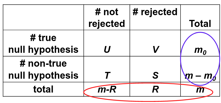

Family-wise error rate (FWER) is the probability of at least one type I error; FWER = P(V > 0)

False discovery rate (FDR) is the expected proportion of type I errors among the rejected hypotheses; FDR = E(V/R)
Assume V/R = 0 when R = 0

Procedures to Control FWER

The general strategy is to adjust p-value of each test for multiple testing; Then compare the adjusted p-values to alpha, so that FWER can be controlled at alpha.

Equivalently, determine the nominal p-value that is required achieve FWER alpha.

Sidák

Sidák adjusted p-value is based on the binomial distribution:

Each test is a trial. Under the null hypothesis, the probability of success is p, the significance level that is used
The probability of at least one success in m trials, each with probability p:
For a test with p-value p_i to adjust for m total tests, the adjusted p-value is p_i^* = 1 - (1 - p_i)^m
This is conservative (over-corrects) when the tests are not independent

Bonferroni

A simplification of Sidák:

Bonferroni adjusted p-value:

p_i^* = mp_i
Over-coirrects (conservative) if the tests are correlated

Below are the individual p-values needed to reject for family-wise significance level=.05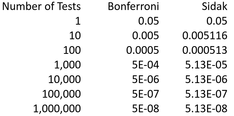

minP

The probability that the minimum p-value from m tests is smaller than the observed p-value when ALL of the tests are NULL.

Equivelent to Sidak adjustment if all tests are independent. But for dependent tests, we don't know the distribution of the p-values under the null hypothesis, so we use permutation to determine the distribution.

Adjusted p-value is the probability that the minimum p-value in a resampled data set is smaller than the observed p-value.

This is less conservative than the above two methods, but the results are equal to Sidak when tests are significant.

Permutation is done under the assumption that the phenotype is independent of the genotypes; and phenotypes are permuted with respect to genotype.
Original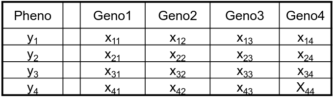

Permuted: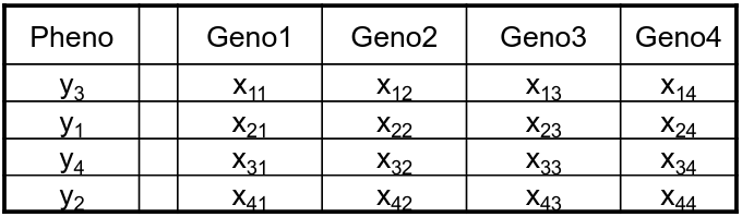

Genotypes from an individual are kept together to preserve LD

Permutation Procedure

Create 1000+ permuted data sets
- Identical to the original except phenotype values have been assigned randomly
Analyze each in exactly the same manner as the original data set
Determine the minimum p-value from each permuted data set
- 1000+ minimum p-values
The minP adjustment: the adjusted p-value is the proportion of minimum p-values that are smaller than the observed p-value.

Permutation is computationally expensive, and in some situations it is not possible at all (related individuals, meta-analysis results).

Alternative

Use the Bonferroni or Sidak correction with the "effective number of independent tests" instead of total number of tests. This reduces the number of tests to account for dependence among test statistics. We must approximate the equivalent number of independent tests.

For a single study you can compute the effective number of independent tests based on the genotype data.

Use the covariance matrix of all the genotypes that you tested
Several approaches have been proppsed to estimate the effective number of tests (m_eff)
Two are best performing:
- Gao X, Starmer J, Martin ER: A multiple testing correction method for genetic association studies using correlated SNPs
- Li J, Ji L: Adjusting multiple testing in multi-locus analyses using the eigenvalues of a correlation matrix

Once you have an estimate of m_eff use it in the Bonferroni or Sidak correction

Another alternative: Extreme Tail Theory Approximation (not covered here)

FWER Summary

Binferroni, Sidak, minP are all single-step adjustments; i.e. all p-values are adjusted in the same manner regardless of their values. This makes them very easy to understand and compute, however it sacrifices power.

Control FWER is very stringent (< 5% chance of a single false positive)

False Discovery Rate (FDR)

Controlling P(V = 0) is too stringent when m is large and you can expect multiple true positives. For better power, control E(V/R) instead.

E(V/R) = the expected proportion of Type I errors among rejected null hypothesises.

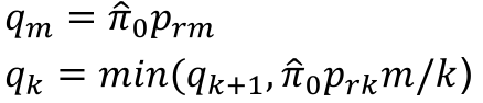
Rank p-values p_r1 <= p_r2 <= ... p_rm
Adjusted p-values
1. p*_rm= p_rm
2. p*_rk = min(p*_rk+1, p_rkm/k)

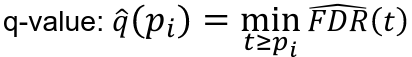
FDR: Q-Value

For an individual hypothesis test, the minimum FDR at which the test may be called significant is the q-value. It indicates the expected proportion of false-positive discoveries among associations with equivalent statistical evidence.

FDR for a specific p-value threshold t: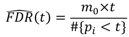
where m₀ = number of true null hypothesis

We can estimate m₀ by m*pi_hat_0; where pi_hat_0 is an estiamte of the proportion of true null hypothesises (could be ~1)

Rank p-values: p_r1 <= p_r2 <= ... p_rm
Estimate the proportion of true null hypothesises pi_hat_0
1. Using pi_hat_0 = 1 leads to conservative q-values estimates equal to the FDR adjusted p-values
2. See suggested approach in Story and Tibshirani (2003)
Compute q-values:
Reject null hypothesis f q-value <= alpha

Which to use?

Bonferroni and Sidak
- Almost no assumptions
- No permutations required
- Use when number of tests is small or power is not an issue, or if a quick computation is needed
- When number of tests is moderate and correlation structure of tests or SNP uses:
  - Extreme tail theory
  - Benferroni adjustment with number of effective independent SNPs
Permutation approach
- Does not assume independence of SNPs
- Use when computationally feasible
FDR or q-value
- Controlling E(V/R) instead of P(V > 0)
- Useful for exploratory analyses with a large number of markers/models/subgroups to test
  - FDR and q-value thresholds are often set higher than traditional (.05) level
- First proposed for analyzing micro-array data
  - Works best when the proportion of null hypotheseses expected to be rejected because they are false is not too small.

Guidelines for Adjusting for Multiple Comparisons

Genome-Wide Association Study (GWAS)
- Must adjust for all tests performed to claim experiment wide significance
- Common strategies:
  - Staged Design:
    - Stage 1: GWAS on subset of available subjects
    - Stage 2: Independent sample/subset, test only the small subset of SNPs that were significant at some level in Stage 1
  - Meta-analysis of multiple studies
    - Each study performs GWAS
    - Results from all studies are combined
  - Combination of these two approaches
Staged GWAS
- Two alternatives for multiple testing correction
  - Replication: Analyze Stage 2 separately, adjust stage 2 for number of tests in stage 2
  - Joint analysis: Analyze stage 1 and 2 jointly for SNPs genotyped in stage 2, adjust joint analysis for all SNPs tested in stage 1
- Usually joint analysis strategy more powerful
  - Joint analysis is more efficient than replication based analysis at two stage genome-wide association studies.
GWAS meta-analysis
- For each SNP, combine results from all studies
- Similar in power to a study with sample size = sum of all sample sizes
- Significance levels appropriate for single GWAS are appropriate for meta-analysis GWAS
Candidate gene studies
- Often we will test SNPs that have already been associated in other independent studies
- Whether the candidate genes were chosen based on prior association, linkage or relevance of any kind
  - must adjusted for all tests performed in your study to claim experiment-wise significance for any one SNP

Overall: we are unlikely to have sufficient power to achieve experiment-wide or genome-wide significance with a single study, large number of SNPs

Best choice is meta-analysis and/or replication using independent studies

When combining studies is not an option, report the most promising results based on p-value and other factors

Make available results from all SNP association analyses so that other investigators can attempt to confirm or repliucate your findings.

Choose a threshold BEFORE looking at the data.

Genomic Control

Genomic control was preposed to measure and adjust for modest population structure within a sample in the context of GWAS

Most SNPs that are tested in a GWAS (which is most) are not associated with the trait
Association tests from random sites in the genome shouhld be distributed as if a set of unassocaited (null) tests
The genomic control inflation factor 𝜆_GC or just 𝜆, is defined as:
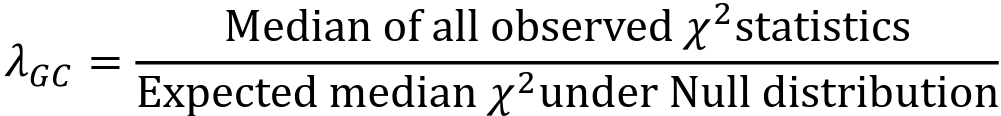
Typically estimated using the entire set of GWAS variants
𝜆 is a measure of the inflation of test statistics in your GWAS
If your study has population structure then the unassociated test statistics will not follow the null distribution.
- On average, each statistic will be a bit "too big"
- The median of the test statistics will be larger than the median test statistic from the null distribution, so 𝜆 > 1
𝜆 can also be used to deflate test statistics so that the observed median matches the expected distribution
- Compute 𝜆
- Divide all test statistics by 𝜆 before computing p-value
GC correction assumes that all the GWAS test statistics are inflated an equal amount

PLINK outputs Z statistics in the STAT column, but 𝜆 is calculated from chi-square test statistics. Z² is a chi-square statistic with 1 degree of freedom. We can transform the p-value from plink into chi using the qchisq() function in R.