Assessing the Genetic Component of a Phenotype

A phenotype is the appearance of an individual, which results from the interaction of the person's genetic makeup and their environment. Phenotypes can be categorical or numerical. If we are interested in the genetic component of a trait  there are different methods we can use for analysis.

We define a trait for analysis, determine what we are interested in studying, and then the methods that need to be used. For example, if we want to know how BMI is linked to gene effects we would need to consider other factors such as age, sex, smoking, etc. Thus, a Multiple Linear Regression might be appropriate, were we can measure the variability of each factor.

Variance of Phenotypic Traits

𝜎²_T = The observed (phenotypic) variability of a trait
𝜎²_T = 𝜎²_G + 𝜎²_E = The phenotypic variability can be partitioned in to variability due to genetic and environmental effects
𝜎²_G = 𝜎²_A + 𝜎²_D = The genetic component can be further partitioned into additive and dominance genetic variance

We can write a model for the trait as:  
T = (A + D) + E = G + E

Assumptions of this model:

• Genetic and environmental factors are uncorrelated
• Standard deviation of trait is the same for all individuals

Additive and Dominance Components

Consider a frequency distribution of trait values for two alleles B and b, where B creates a high trait value and b creates a low trait value on a continuous scale which is shifted so that the midpoint between the mean of BB (+a) and bb (-a) is 0:

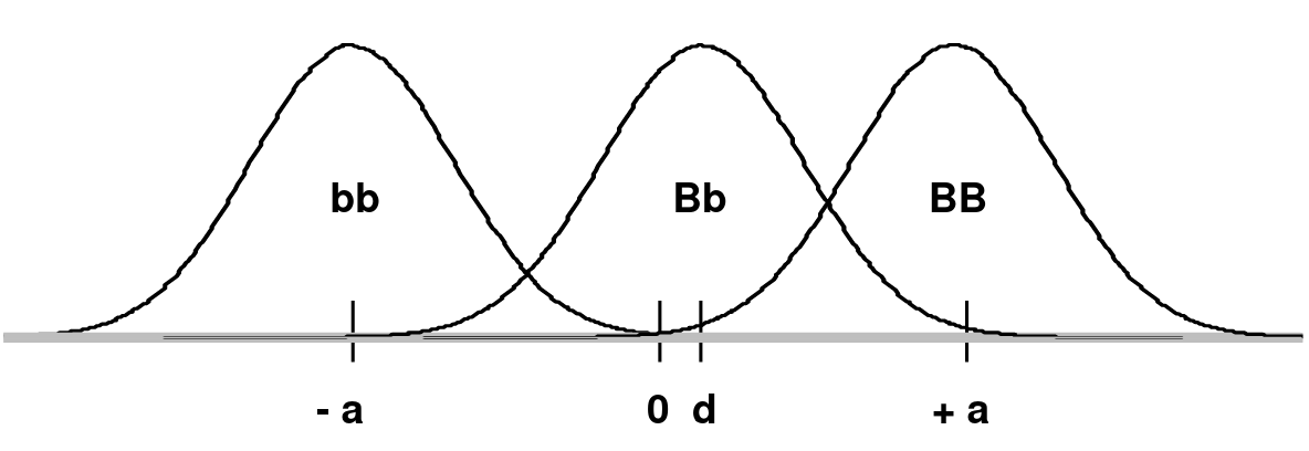
d is the mean of the Bb group

In an additive model d = 0 (no dominance; dominance variance = 0)
In a recessive model: d = -a    (Bb would overlap the bb distribution)
In a dominant model d = +a   (Bb would overlap the BB distribution)

The degree of dominance can be defined as d/a

Heritability

The heritability of a trait is the proportion of total phenotypic variance that is due to genetic effects.

Heritability can be defined as:

h²    =    𝜎²_G /  𝜎²_T     =   ( 𝜎²_A + 𝜎²_D ) / ( 𝜎²_A + 𝜎²_D + 𝜎²_E )

The above formula is also called Broad sense hertiability. Narrow sense heritability (just the additive component): 

h_n²    =  𝜎²_A  / 𝜎²_T

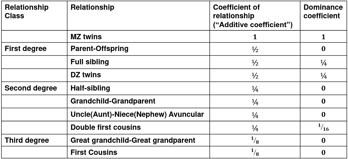
We use the expected resemblance among relatives to estimate h². It is a function of covariance between relatives and coefficient of relationship (AKA "Additive coefficient")

The additive coefficient of a relationship C is the expected proportion of alleles shared IBD by a relative pair, defined as:

C = 2^-R, where R is the degree of relationship

• R = 0: MZ twins -> C = 1
• R = 1: 1st degree relationship; sib, parent-offspring -> C = 1/2
• R = 2: 2nd degree relatives: half-sibs, grandparent-grandchild, avuncular
• R = 3: 1st cousins

Recall sharing a allele Identical-By-Descent means relatives who share the exact same copy of an allele by inheritance.

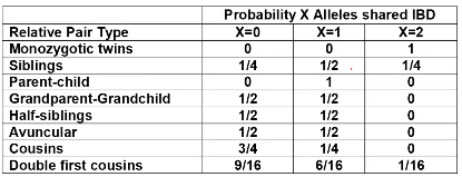
The additive coefficient is expected proportion of alleles shared IBD by the pair, so we can also define it as

p(x) = x/2 = the proportion of shared alleles

For example, the parent child relationship would have a additive coefficient of 0*(0/2) + 1*(1/2) + 0*(2/2) = 1/2

The kinship coefficient is the probability that a randomly selected pair of alleles from a individual is IBD. It is always half of the coefficient of relationship.

Estimating Heritability

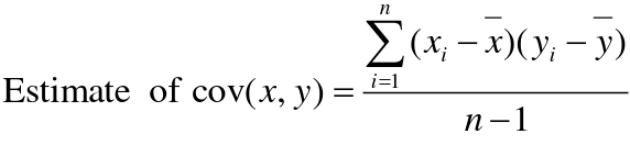
Using Co-variance

Recall the properties of covariance:

• Cov(X,Y) = Cov(Y,X)
• Cov(X, X) = var(X)
• Cov(X + Y, Z) = Cov(X, Z) + Cov(Y, Z)
• Cov(cX, Y) = c*Cov(X,  Y); where c is some constant
• The unit of covariance is xy
• Positive covariance: Value of x tends to be high when value of y is high
• Negative covariance: Value of x tends to be high when value of y is low

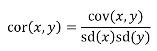
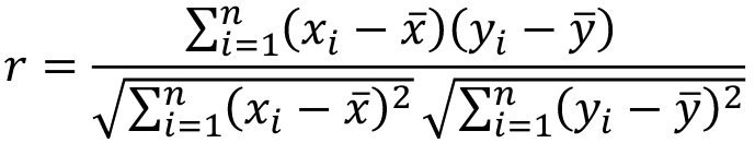
A standardized measure of covariance is correlation which is a scale of -1 to 1

We can use the properties of covariance to determine the covariance between quantitative measure on a parent and an offspring. This folows the same T = (A + D) + E = G + E concept as above:

Cov(Parents, Offsrping) = Cov (A_p + D_p + E_p, A_o + D_o + E_o)

In this example, we can break this down into:

• Cov (A_p, A_o) = Additive covariance, offspring always inherits exactly 1 allele from parent so = (1/2)𝜎²_A 
  
• Cov (E_p, E_o),  covariance of environmental component between parent and offspring is assumed to be 0
  
• Cov (D_p, D_o) = Since offspring do not inherit pairs of alleles the dominance environmental component is also 0
  
• The cross terms, Cov(A, D) and etc. which we assume to be 0

Note: This only works if the assumptions of independence is true and standard deviation is the same for all individuals.

Since we are assuming standard deviation is the same across generations we can write hieritability between parent and offspring as a product of correlation:

h_n² =  𝜎²_A  / 𝜎²_T = 2 * Cov(parent, offspring) / SD(parent)*SD(child) = 2 * Cor(parent, offspring)

Thus, we can estimate narrow-sense heritability using 2 times the observed correlation between parents and offspring.

Using Linear Regression

Alternatively, we can use the linear regression coefficient to estimate heritability. Where Y is offspring and X is parent:

𝑌 = 𝛼 + 𝛽𝑋 + 𝐸

 𝛽_hat ~ cor(X, Y) x SD(Y)/SD(X)

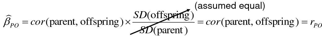
h_n² = 2*r_PO = 2*𝛽_hat_PO

Note that the estimate obtained from beta may differ from the estimate obtained from r if the standard deviations of parents and offspring are not equal.

If both parents are available we can regress the offspring value of the mean parental phenotype value:

h² = 𝛽_hat_MO  

Beta estimates heritability directly in the average parent version. I'm not going show the math here, but know this is in part due to SD(average parent) = SD(parent) / sqrt(2)

Example with Sibling Pairs

Looking at the relationship table above in the siblings row: additive coefficient is 1/2 and dominance coefficient 1/4. If data is available on N sibling pairs only:

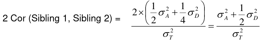
Cov(Sibling 1. Sibling 2) = (1 / 2) 𝜎²_A + (1 / 4) 𝜎²_D 

If 𝜎²_D   = 0, 2 times the intraclass correlation (ICC) is an estimate of heritability: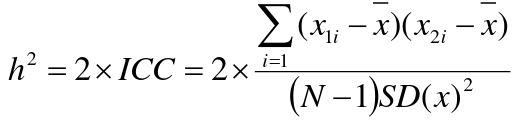
Where x and SD(x) are computed combining data on all siblings.

If 𝜎²_D  does not equal 0, this estimate is between the narrow and broad heritability because:

Intraclass Correlation Vs. Pearson (Product-Moment) Correlation

When pairs consist of individuals of two different classes (grandparent-grandchild, parent-offspring) we call this pairwise correlation and we can use a simple Pearson correlation coefficient:

But when the pairs have no obvious order (siblings or cousins), the intraclass correlation is used:

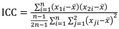
where n is the number of pairs and x_bar is the mean value across all individuals

The main difference between the product-moment correlation and ICC:

• ICC: SD in the denominator is pooled across individuals
  
• Pearson: SD for the two types of relatives are computed separately

ICC can be extended to sets of 3 or more. The formula for ICC is:

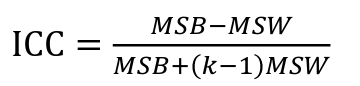
k = number of siblings per sibship
MSB = Mean Square Between (model)
MSW = Mean Square Within (error)
If the sibships are of unequal size using the average sibship size will provide an approximate h² estimate

h² = 2 * ICC

Twin Studies

Monozygotic twins are genetically identical and dizygotic twins are genetic the same as a full sibling, sharing half their genes on average. A common estimate of heritability in studies with both mono and dizygotic twins can estimate it as:

h² = 2 * (ICC_MZ - ICC_DZ)

If 𝜎²_D  does not equal 0, this estimate is greater than both the narrow and broad heritability because:

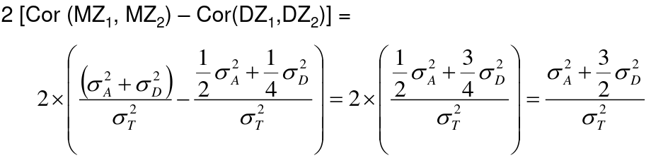
This is in part because we cannot assume there is no shared environmental variance in siblings and especially twins.

Notes on Estimating Heritability

• We can obtain different estimates using different subsets of data
• Differences in estimates may be due to "sampling variation"
• If the dominance variance is not 0, some differences may be expected
  • Siblings and twins incorporate dominance variance; parent-offspring do not
• Siblings and twins tend to share environment/exposure factors
• We may get smaller estimates with pairs that are more similar (Age, weight, etc)
• Precision of heritability estimates depends on the SE of the correlation coefficient or regression coefficient used for the estimation
• Large sample sizes are needed to get precises measures of heritability
• Heritability is a ratio of variances, not an average
• Law of large numbers does not necessarily apply here, heritability does not necessarily follow a normal distribution
• Maximum likelihood approach can be used to estimate  𝜎²_{T ,} 𝜎²_A, and 𝜎²_D -- and can also estimate shared environments when we are not assuming it to be 0 

We can estimate the linear mixed effects (variance component model):

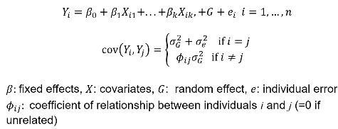
In which case we would estimate heritability as 𝜎²_G and test H0: 𝜎²_G  = 0

Heritability Summary

• Heritability is a population parameter, defined as the proportion of trait variance explained by additive genetic factors
  • Estimates of h² are usually based on resemblance between relatives
  • Highly heritable -> close relatives should be more correlated 
• Heritability may differ by population
  • h² depends on both 𝜎²_T  and 𝜎²_A
• h² estimates using close and distant relatives should be similar
  • Estimates bases on twins, sibs and cousin pairs estimate the same population parameter (unless there is dominance variance)
• If a trait is not heritable (h² = 0), we do not expect close relatives to be more correlated than distance relatives
• Heritability is generally computed for quantitative traits with analysis of variance, but can also be estimated for discrete traits
  • Liability, or predisposition to disease, is measured on a quantitative scale
  • Threshold model: trait present if liability to disease exceeds a certain threshold
  • Heritability measures the liability between relatives
  • There is specialized software for calculating this
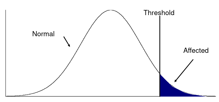
  • Referred to as the "latent variable" model, we can observe whether an individual has cross the threshold

Recurrence Risk Ratio

Recurrence risk ratio assess familial aggregation of dichotomous traits (diseases).  𝜆_𝑅 denotes relative risk with a subscript indicating the specific type of relative examined.

A proband is a subject selected for a study due to disease status. In familial disease studies, it is the affected subject that brought the family into the study

𝜆_𝑅 = 𝐾_𝑅/𝐾
𝐾_𝑅 = P(disease | relative of type R is affected) =  the proportion (prevalence) of relatives of affected probands that are affect with disease
K = the proportion of affected individuals in the general population

General rule:

• If a trait is generic 𝜆_𝑅 should decrease as degree of relationship increases
• Differences in shared environment may lead to differences in 𝜆_𝑅 for different relative types of the same degree
• 𝜆_𝑅 may be greater than 1 when the trait does not have a genetic component due to a shared enviornment