Mutiple Linear Regression and Estimation

Multiple Linear Regression analysis can be looked upon as an extension of simple linear regression analysis to the situation in which more than one independent variables must be considered.

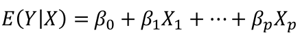
The general model with response Y and regressors X₁, X₂,... X_p:

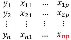
Suppose we observe data for n subjects with p variables. The data might be presented in a matrix or table like:

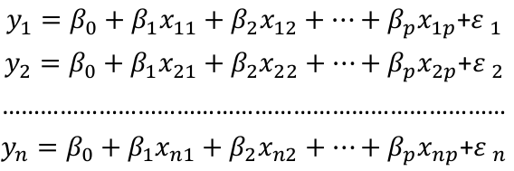
We could then write the model as:

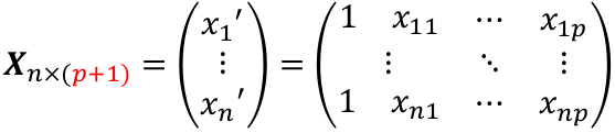
We can think of Y and E as (n x 1) vectors when transposed, and β as a ((p + 1) x 1) vector. p +1 is number of predictors + the intercept. Thus X would be:

The general linear regression may be written as:

Or y_i = x_i^|*β + ∈_i

The model is represented as the systematic structure plus the random variation with n dimensions = (p + 1) + { n - (p + 1 ) }

Ordinal Least Squares Estimators

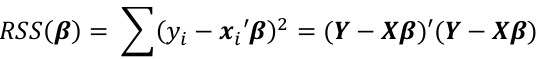
The least squares estimate β_hat of β is chosen by minimizing the residual sum of squares function:

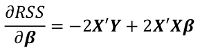
By differentiating with respect to β_i and solve by setting equal to 0:

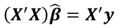
The least squares estimate of β_hat of β is given by:

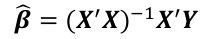
and if the inverse exists:

Fitted Values and Residuals

The fitted values are represetned by Y_hat = X*β_hat

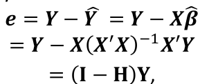
where the hat matrix is defined as H = X(X^|X)^-1X^|

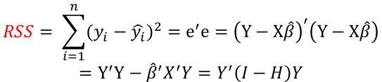
The residual sum of squares (RSS):

Gauss-Markov Conditions

In order for estimates of β to have some desirable statistical properties, we need a set of assumptions referred to as the Gauss-Markov conditions; for all i, j = 1... n

E[∈_i] = 0
E[∈_i²] = 𝜎²
E[∈_i∈_j] = 0, where i != j

Or we can write these in matrix notation as: E[∈] = 0, E[∈∈^|] = 𝜎²*I

The GM conditions imply that E[Y] = Xβ and cov(Y) = E[(Y-Xβ)(Y-Xβ)^|] = E[∈∈^|] = ∈

Under the GM assumptions, the LSE are the Best Linear Unbiased Estimators (BLUE). In this expression, "best" means minimum variance and linear indicates that the estimators are linear functions of y.

The LSE is a good choice but it does require the errors are uncorrelated and have equal variance. Even if the errors behave, then nonlinear or biased estimates may work better.

Estimating Variance

By definition:

We can estimate variance by an average from the sample:

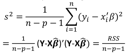
Under GM conditions, s² is an unbiased estimate of variance.

Total Sum of Squares

Total sum of squares is Syy = SSreg + RSS

The corrected total sum of squares with n-1 degrees of freedom:

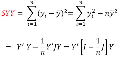
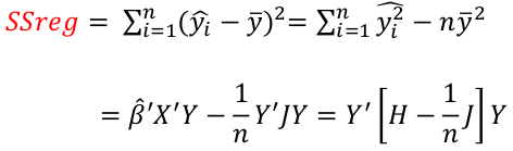
where J is an n x n matrix of 1s and H = X(X^|X)^-1X^|

Regression and Residual Sum of Sqaures

Regression sum of squares represent the number of X variables:

Residual Sum of Squares with n - (p + 1) degrees of freedom:

F Test for Regression Relation

To test whether there is a regression relation between Y and a set of variables X, use the hypothesis test:

𝐻0 : 𝛽1 = 𝛽2 = 𝛽3 = ⋯ = 𝛽𝑝 = 0 v.s. 𝐻1 : not all 𝛽𝑘 = 0, 𝑘 = 1, … , 𝑝

We use the test statistic:

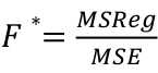
The chances of a Type I error is alpha, our degrees of freedom is n - p -1

The Coefficient of Determination

Recall this measures the model of fit by the proportionate reduction of total variation in Y associated with the use of the set of X variables.

R² = SSreg / Syy = 1 - RSS / Syy

In a multi-linear regression we must adjust the coefficient by the associated degrees of freedom:

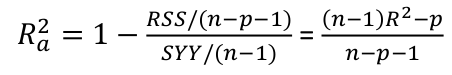
Add more independent variables to the model can only increase R², but R²_alpha may become smaller when more independent variables are introduced, as the decrease in RSS may be offset by the loss of degrees of freedom.

T Tests and Intervals

Tests for β_k are pretty standard:

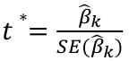
With the rejection rule of 𝑡 >= t(1 − 𝛼/2; 𝑛 − 𝑝 − 1)

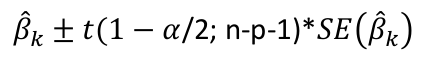
And likewise confidence limits for β_k and 1 - alpha confidence