Midterm Cheat Sheet

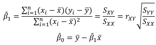
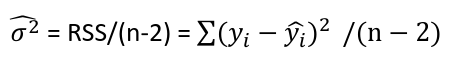
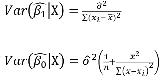
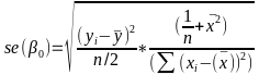
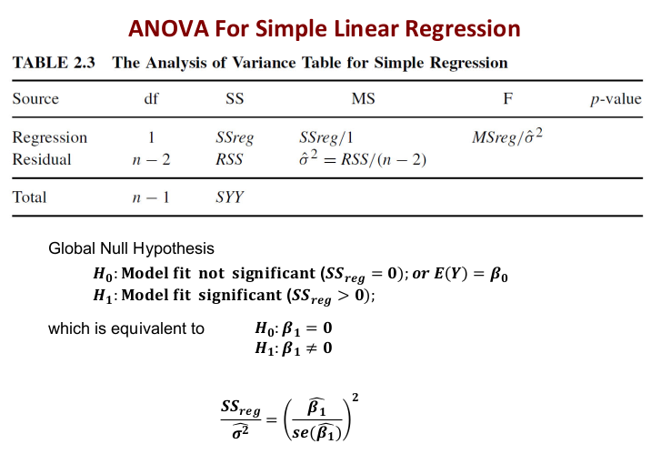
Linear Regression

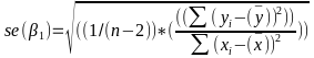
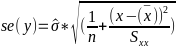
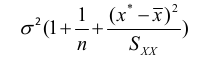
Predicting a CI new obs adds a 1 to se(y):

𝛽₀ + 𝛽₂x +/- t*

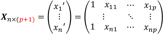
Multiple Linear Regression and Estimation

𝐻0 : 𝛽1 = 𝛽2 = 𝛽3 = ⋯ = 𝛽𝑝 = 0  
v.s.  𝐻1 : not all 𝛽𝑘 = 0, 𝑘 = 1, … , 𝑝

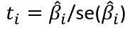
rejection rule of 𝑡 >= t(1 − alpha/2; 𝑛 − 𝑝 − 1)

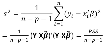
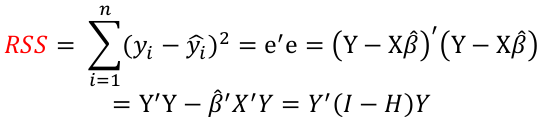
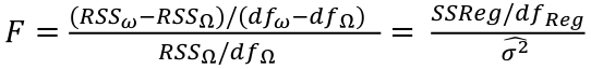
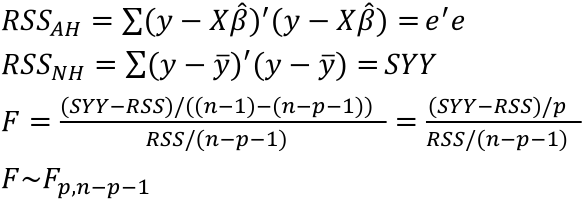
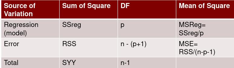
Model Fitting: Inference

df_Ω = n - p, and df_𝜔 = n – q

Reject the null hypothesis if F > Fα p - q, n – p

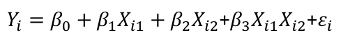
Dummy Variables and Analysis of Covariance
Consider a Xi2 for which is 0 for – and 1 for +:

An interaction between Xi1 and Xi2:

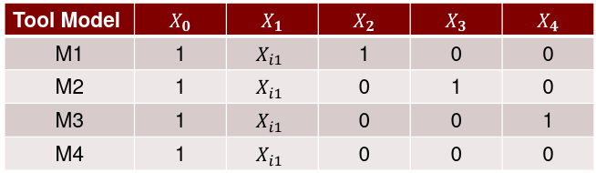
A model with multiple categorical variables:

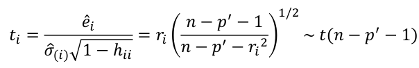
Regression Diagnostics
Assumptions:
    • Error:  ~ N(0, SD2I); 
        ◦ Independent
        ◦ Equal Variance
        ◦ Normally Distributed
    • Model: E[y] = Xβ is correct
    • Unusual observations
      
Leverage Points: data point with unusual x-value

      The Hat Matrix – n*n matrix
h_ii is the leverage of the i^th case
leverage > 2p’/n should be looked at closely

Outliers: Unusual observation on x or y axis

Calculate the t-test and compare abs with limit:
abs(qt(.05/(n*2), df = n - pprime - 1, lower.tail = T))

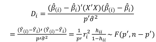
Influential Points: causes changes to regression
    Difference in Fits:

with a threshold of

Where p’ is the number of parameters 

    Cook's Distance:

with a threshold of
Di > 4/n should be looked at
Di > .5 possible influence
Di >= 1 very influential

Error: a plot of e_hat should
    • have constant variance
    • have no clear pattern
    • H0: residuals are normal

Shapiro-Wilk normality test

H0: Residuals are normally distributed

Bonferroni Correction: Divide alpha by n

Variable Selection

Backwards Elimination:

1. Start model with all the predictors

2. Remove the predictor with highest p-value greater than alpha

3. Refit the model

4. Remove the remaining least significant predictor provided its p-value is greater than alpha

5. Repeat 3 and 4 until all "non-significant" predictors are removed

Cutoff p significance can be 15-20% for testing

Forward Selection:

1. Start model with no predictors

2. For predictors not in the model, check the p-value if they are added to the model. We choose the one with lowest p-value less than alpha

3. Continue until no new predictors can be added

Stepwise regression: A combination of the two

Selection Criteria:
Akaike Information Criterion (AIC): 
    • -2 max log-likelihood + 2p' 
    • n*log(RSS/n) + 2p'
Bayes Information Criterion (BIC): 
    • -2 max log-likelihood + p' log(n) 
    • n*log(RSS/n) + log(n) * p' 
Adjusted R2:
R² = 1 – RSS/SSY

Mallow’s C_p Statistic: Avg MSE of prediction

If a p-predictor fits then:

We desire models with small p and Cp around or less than p

# Model with only beta_0

sr_lm0 <- lm(y ~ 1, data=sr)

# Full model

sr_lm1 <- lm(y ~ ., data=sr)

sr_syy <- sum((savings$sr - mean(savings$sr))^2)

sr_rss <- deviance(sr_lm1)

# F = ((SYY -RSS)/((n-1) - (n-2))) / (RSS / (n - 1))

sr_num <- (sr_syy - sr_rss)/(df.residual(sr_lm0) - df.residual(sr_lm1))

sr_den <- sr_rss / df.residual(sr_lm1)

sr_f <- sr_num / sr_den

# dfΩ = n - p, and df𝜔 = n - q

pf(sr_f, df.residual(sr_lm0) - df.residual(sr_lm1), df.residual(sr_lm1), lower.tail = F)

# β=(X^I X)⁻¹ X^IY

beta <- solve(t(x)%*%x)%*%(t(x)%*%y)

# Pearson's

cor(lin_reg$fitted.values, lin_reg$residuals, method="pearson")

# Stratify variables by a factor

by(depress, depress$publicassist, summary)

# Welsh's Two Sample T-test

# For difference in means

t.test(assist$cesd, noassist$cesd) # or t.test(data.y ~ factor)

# CI of LS means based on covariates

library(lsmeans)

lsmeans(reg, ~Type)

# Apply a mean function to an array

# split on a factor

tapply(assist$cesd, assist$assist, mean)

# When a regression factor has

# more than two categories

reg <- lm(Pulse1 ~ Height + Sex + Smokes + as.factor(Exercise))

# Cook's Distance

cook <- cooks.distance(reg)

cook[cook > 4/n]

# Shapiro Test for normallity

shapiro.test(reg$residuals)

# Studentized residuals

stud <- rstudent(reg)

# Threshold for lower tail of

# studentized resids with correction

lim = abs(qt(.05/(n*2), df = n - pprime - 1, lower.tail = T))

stud[which(abs(stud) > lim)]

# Hat values

hat <- hatvalues(reg)

lev <- 2 * pprime / n

hat[hat > lev]

# Forward selection

forward <- ~ year + unemployed + femlab + marriage + birth + military

m0 <- lm(divorce ~ 1, data = usa)

reg.forward.AIC <- step(m0, scope = forward, direction = "forward", k = 2)

n <- nrow(usa)

# AIC = n*log(RSS/n) + 2p'

n*log(162.1228/n)+2*6

extractAIC(reg.forward.AIC, k=2)

# BIC

reg.forward.BIC <- step(m0, scope = forward, direction = "forward", k = log(n))

extractAIC(reg.forward,k=log(n))

# BIC = n*log(RSS/n) + p'*log*n)

n*log(162.1228/n)+6*log(n)

library(leaps)

leaps <- regsubsets(divorce ~ .)

rs <- summary(leaps)

par(mfrow=c(1,2))

plot(2:7, rs$cp, xlab="No. of parameters", ylab="Cp Statistic")

abline(0,1)