| **Linear Regression** [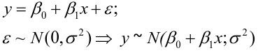](https://bookstack.mitchellhenschel.com/uploads/images/gallery/2022-10/image-1666104229251.png) [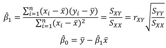](https://bookstack.mitchellhenschel.com/uploads/images/gallery/2022-10/image-1666104239088.png) [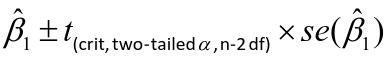](https://bookstack.mitchellhenschel.com/uploads/images/gallery/2022-10/image-1666104245811.png) [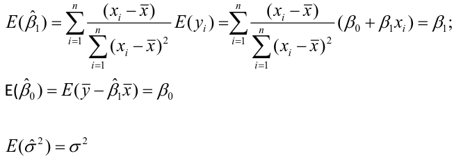](https://bookstack.mitchellhenschel.com/uploads/images/gallery/2022-10/image-1666104252727.png) [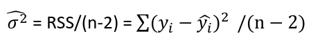](https://bookstack.mitchellhenschel.com/uploads/images/gallery/2022-10/image-1666104260540.png) [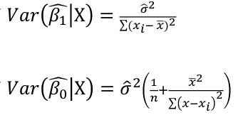](https://bookstack.mitchellhenschel.com/uploads/images/gallery/2022-10/image-1666104271056.png) [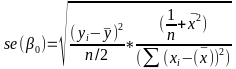](https://bookstack.mitchellhenschel.com/uploads/images/gallery/2022-10/image-1666104276418.png) [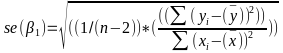](https://bookstack.mitchellhenschel.com/uploads/images/gallery/2022-10/image-1666104282605.png) [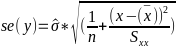](https://bookstack.mitchellhenschel.com/uploads/images/gallery/2022-10/image-1666104287023.png) Predicting a CI new obs adds a 1 to se(y): 𝛽0 + 𝛽2x +/- t\*[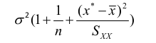](https://bookstack.mitchellhenschel.com/uploads/images/gallery/2022-10/image-1666104297248.png) | **Multiple Linear Regression and Estimation** [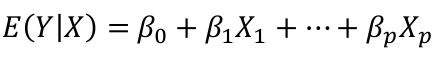](https://bookstack.mitchellhenschel.com/uploads/images/gallery/2022-10/image-1666104323618.png) [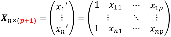](https://bookstack.mitchellhenschel.com/uploads/images/gallery/2022-10/image-1666104327905.png) [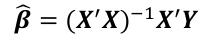](https://bookstack.mitchellhenschel.com/uploads/images/gallery/2022-10/image-1666104332246.png) [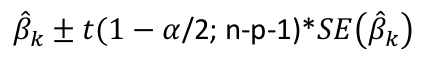](https://bookstack.mitchellhenschel.com/uploads/images/gallery/2022-10/image-1666104336362.png) [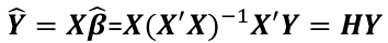](https://bookstack.mitchellhenschel.com/uploads/images/gallery/2022-10/image-1666104345652.png) [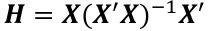](https://bookstack.mitchellhenschel.com/uploads/images/gallery/2022-10/image-1666104350789.png) [](https://bookstack.mitchellhenschel.com/uploads/images/gallery/2022-10/image-1666104355280.png) [](https://bookstack.mitchellhenschel.com/uploads/images/gallery/2022-10/image-1666104359234.png) [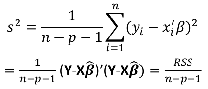](https://bookstack.mitchellhenschel.com/uploads/images/gallery/2022-10/image-1666104363437.png) [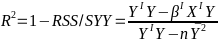](https://bookstack.mitchellhenschel.com/uploads/images/gallery/2022-10/image-1666290673808.png) [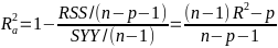](https://bookstack.mitchellhenschel.com/uploads/images/gallery/2022-10/image-1666290691336.png) 𝐻0 : 𝛽1 = 𝛽2 = 𝛽3 = ⋯ = 𝛽𝑝 = 0 v.s. 𝐻1 : not all 𝛽𝑘 = 0, 𝑘 = 1, … , 𝑝 [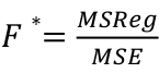](https://bookstack.mitchellhenschel.com/uploads/images/gallery/2022-10/image-1666104389032.png)[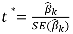](https://bookstack.mitchellhenschel.com/uploads/images/gallery/2022-10/image-1666104395117.png) rejection rule of 𝑡 >= t(1 − alpha/2; 𝑛 − 𝑝 − 1) [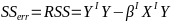](https://bookstack.mitchellhenschel.com/uploads/images/gallery/2022-10/image-1666104407108.png) [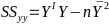](https://bookstack.mitchellhenschel.com/uploads/images/gallery/2022-10/image-1666104410593.png) [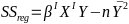](https://bookstack.mitchellhenschel.com/uploads/images/gallery/2022-10/image-1666104415116.png) [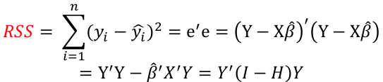](https://bookstack.mitchellhenschel.com/uploads/images/gallery/2022-10/image-1666104423017.png) |
| **Model Fitting: Inference** [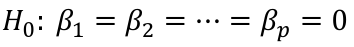](https://bookstack.mitchellhenschel.com/uploads/images/gallery/2022-10/image-1666104576887.png) dfΩ = n - p, and df𝜔 = n – q [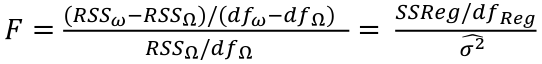](https://bookstack.mitchellhenschel.com/uploads/images/gallery/2022-10/image-1666138531298.png) Reject the null hypothesis if F > Fα p - q, n – p [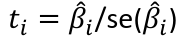](https://bookstack.mitchellhenschel.com/uploads/images/gallery/2022-10/image-1666104643517.png) [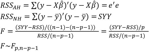](https://bookstack.mitchellhenschel.com/uploads/images/gallery/2022-10/image-1666138340542.png) | **Dummy Variables and Analysis of Covariance** Consider a Xi2 for which is 0 for – and 1 for +: [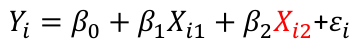](https://bookstack.mitchellhenschel.com/uploads/images/gallery/2022-10/image-1666104607845.png) An interaction between Xi1 and Xi2: [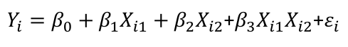](https://bookstack.mitchellhenschel.com/uploads/images/gallery/2022-10/image-1666104615922.png) A model with multiple categorical variables: [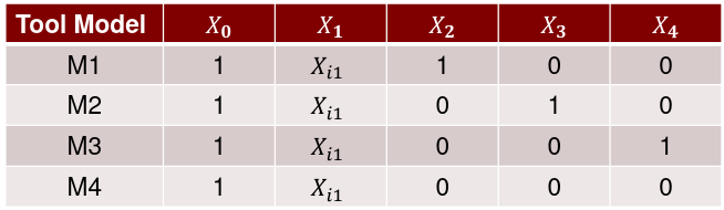](https://bookstack.mitchellhenschel.com/uploads/images/gallery/2022-10/image-1666104625980.png) [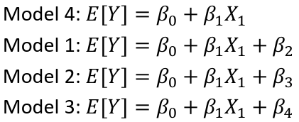](https://bookstack.mitchellhenschel.com/uploads/images/gallery/2022-10/image-1666104633030.png) |
| **Regression Diagnostics** Assumptions: • Error: ~ N(0, SD2I); ◦ Independent ◦ Equal Variance ◦ Normally Distributed • Model: E\[y\] = Xβ is correct • Unusual observations Leverage Points: data point with unusual x-value [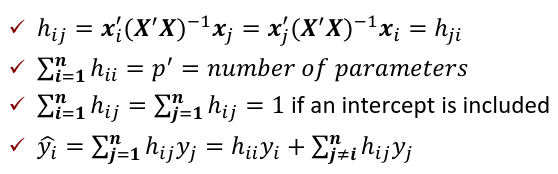](https://bookstack.mitchellhenschel.com/uploads/images/gallery/2022-10/image-1666104773344.png) The Hat Matrix – n\*n matrix hii is the leverage of the ith case leverage > 2p’/n should be looked at closely Outliers: Unusual observation on x or y axis [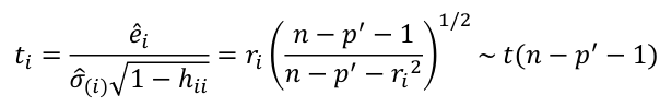](https://bookstack.mitchellhenschel.com/uploads/images/gallery/2022-10/image-1666104790374.png) Calculate the t-test and compare abs with limit: abs(qt(.05/(n\*2), df = n - pprime - 1, lower.tail = T)) | Influential Points: causes changes to regression Difference in Fits: [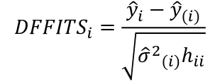](https://bookstack.mitchellhenschel.com/uploads/images/gallery/2022-10/image-1666104815733.png) with a threshold of [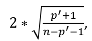](https://bookstack.mitchellhenschel.com/uploads/images/gallery/2022-10/image-1666104825747.png) Where p’ is the number of parameters Cook's Distance: [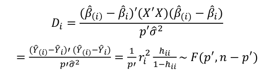](https://bookstack.mitchellhenschel.com/uploads/images/gallery/2022-10/image-1666104834542.png) with a threshold of Di > 4/n should be looked at Di > .5 possible influence Di >= 1 very influential Error: a plot of e\_hat should • have constant variance • have no clear pattern • H0: residuals are normal Shapiro-Wilk normality test H0: Residuals are normally distributed Bonferroni Correction: Divide alpha by n |
| **Variable Selection** Backwards Elimination: 1. Start model with all the predictors 2. Remove the predictor with highest p-value greater than alpha 3. Refit the model 4. Remove the remaining least significant predictor provided its p-value is greater than alpha 5. Repeat 3 and 4 until all "non-significant" predictors are removed Cutoff p significance can be 15-20% for testing Forward Selection: 1. Start model with no predictors 2. For predictors not in the model, check the p-value if they are added to the model. We choose the one with lowest p-value less than alpha 3. Continue until no new predictors can be added Stepwise regression: A combination of the two | Selection Criteria: Akaike Information Criterion (AIC): • -2 max log-likelihood + 2p' • n\*log(RSS/n) + 2p' Bayes Information Criterion (BIC): • -2 max log-likelihood + p' log(n) • n\*log(RSS/n) + log(n) \* p' Adjusted R2: R2 = 1 – RSS/SSY [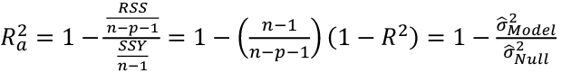](https://bookstack.mitchellhenschel.com/uploads/images/gallery/2022-10/image-1666202623504.png) Mallow’s Cp Statistic: Avg MSE of prediction [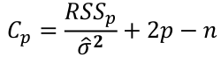](https://bookstack.mitchellhenschel.com/uploads/images/gallery/2022-10/image-1666202639730.png)If a p-predictor fits then: [](https://bookstack.mitchellhenschel.com/uploads/images/gallery/2022-10/image-1666202661358.png) We desire models with small p and Cp around or less than p |
| \# Model with only beta\_0 sr\_lm0 <- lm(y ~ 1, data=sr) \# Full model sr\_lm1 <- lm(y ~ ., data=sr) sr\_syy <- sum((savings$sr - mean(savings$sr))^2) sr\_rss <- deviance(sr\_lm1) \# F = ((SYY -RSS)/((n-1) - (n-2))) / (RSS / (n - 1)) sr\_num <- (sr\_syy - sr\_rss)/(df.residual(sr\_lm0) - df.residual(sr\_lm1)) sr\_den <- sr\_rss / df.residual(sr\_lm1) sr\_f <- sr\_num / sr\_den \# dfΩ = n - p, and df𝜔 = n - q pf(sr\_f, df.residual(sr\_lm0) - df.residual(sr\_lm1), df.residual(sr\_lm1), lower.tail = F) \# β=(XI X)−1 XIY beta <- solve(t(x)%\*%x)%\*%(t(x)%\*%y) \# Pearson's cor(lin\_reg$fitted.values, lin\_reg$residuals, method="pearson") \# Stratify variables by a factor by(depress, depress$publicassist, summary) \# Welsh's Two Sample T-test \# For difference in means t.test(assist$cesd, noassist$cesd) \# or t.test(data.y ~ factor) \# CI of LS means based on covariates library(lsmeans) lsmeans(reg, ~Type) \# Apply a mean function to an array \# split on a factor tapply(assist$cesd, assist$assist, mean) \# When a regression factor has \# more than two categories reg <- lm(Pulse1 ~ Height + Sex + Smokes + as.factor(Exercise)) | \# Cook's Distance cook <- cooks.distance(reg) cook\[cook > 4/n\] \# Shapiro Test for normallity shapiro.test(reg$residuals) \# Studentized residuals stud <- rstudent(reg) \# Threshold for lower tail of \# studentized resids with correction lim = abs(qt(.05/(n\*2), df = n - pprime - 1, lower.tail = T)) stud\[which(abs(stud) > lim)\] \# Hat values hat <- hatvalues(reg) lev <- 2 \* pprime / n hat\[hat > lev\] \# Forward selection forward <- ~ year + unemployed + femlab + marriage + birth + military m0 <- lm(divorce ~ 1, data = usa) reg.forward.AIC <- step(m0, scope = forward, direction = "forward", k = 2) n <- nrow(usa) \# AIC = n\*log(RSS/n) + 2p' n\*log(162.1228/n)+2\*6 extractAIC(reg.forward.AIC, k=2) \# BIC reg.forward.BIC <- step(m0, scope = forward, direction = "forward", k = log(n)) extractAIC(reg.forward,k=log(n)) \# BIC = n\*log(RSS/n) + p'\*log\*n) n\*log(162.1228/n)+6\*log(n) library(leaps) leaps <- regsubsets(divorce ~ .) rs <- summary(leaps) par(mfrow=c(1,2)) plot(2:7, rs$cp, xlab="No. of parameters", ylab="Cp Statistic") abline(0,1) |