Principal Component Analysis

The goal of supervised learning methods (regression and classification) is to predict outcome/response variable Y using a set of p features (X1, X2... Xp) measured on n observations. We train the machine on 'labeled' data to predict outcomes for unforeseen data.

Unsupervised learning is a set of tools (principle component analysis and clustering) intended to explore only a set of features (X1, X2... Xp) and to discover interesting things about these features. This is often performed as part of an exploratory data analysis.

The challenge of unsupervised learning is that is is more subjective than supervised learning, as there is no simple goal for the analysis such as prediction of a response.

Principle Component Analysis (PCA)

Visualize n observations with measurements on a set of p features as part of an exploratory data analysis. Do this by examining 2-dimensional scatterplots. PCA produces a low-dimensional representation of a dataset that contains as much variation as possible.

Input of PCA is a data matrix in which the columns are centered to have mean 0. Typically the columns represent variables (age, weight, etc) and rows represent different subjects.

Output of PCA is a data matrix Y in which the columns are linear transformations of the columns of X, and they are uncorrelated.

In general the columns has n rows and p columns (variables).

Method

PCA uses orthogonal transformation to convert the columns of X into new variables called principal components that are:

• Linear combinations of the original variables
• Uncorrelated
• Sorted so that the first PC has the largest variance and the rest are descending
• We can have at most as many PCs as columns, assuming p < n

The first principal component is the normalized linear combination of the vectors x1, ..., xp that has the largest variance. By normalized we mean: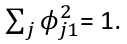

Where the theta elements of the above are loadings of the first principal component. We constrain the loadings so that their sum of squares is equal to one, since otherwise setting these elements to be arbitrarily large in absolute value could result in an arbitrarily large variance.

Calculating the First Principal Component

Assuming that the variables Xi are centered, we search for the loadings that maximize the sample variance of teh first PC, subject to the constraint above that sum of theta_j1^2 = 1.

We refer y11, y21, ..., yn1 as the scores or realized values of the first principal component where:

The average of yi1 (the scores of the first PC) is 0 since it is centered. The sample variance of the values of the n values of yi1 is: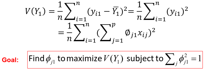

The loading vector theta_1 with elements theta_11, theta_21, ..., theta_p1 defines a direction in feature space along which the data vary the most.

If we project the n data points x1, x2, ..., xn onto this direction, the projected values are the principal component scores y11, y21, ..., yn1 themselves.

Calculation of the Second Principal Component

After we find 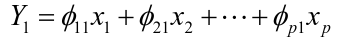 we can calculate the second PC:

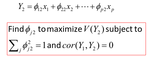
And so on until all PCs are found. These calculations can be done using the "singular value decomposition".

In R the 'prcomp()' function computes principal components by using a singular value decomposition.

The advantage of using PCA is that we hope to end up with a number of components that is smaller than the number of variables p.

We can use PCA for data reduction techniques. If 2 or 3 PCs explain a large portion of the total variance, then we can use these 2 or 3 variables for analysis rather than the whole set.

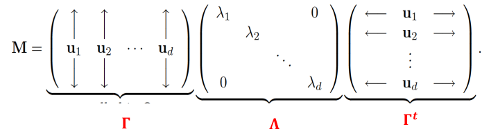
Spectral Decomposition

The spectral decomposition recasts a matrixx in terms of it eignenvalues and eigenvectors. The representation turns out to be very useful.

Let M be a real symmetric d x d matrix with eigen values lambda_1, lambda_2, ..., lambda_d and corresoinding orthonormal eigenvectors u1, u2, ..., ud then:

R Code

### Example 1
head(USArrests)
dim(USArrests)
sqrt(apply(USArrests,2,var))

plot(USArrests)
# compute principal components
pca1 <- prcomp(USArrests, scale=T)
pca1
(13.2 -mean(USArrests$Murder))/sqrt(var(USArrests$Murder))*( -0.5358995) +
  (236-mean(USArrests$Assault))/sqrt(var(USArrests$Assault))*(-0.5831836) +
  (58-mean(USArrests$UrbanPop))/sqrt(var(USArrests$UrbanPop))*(-0.2781909) +
  (21.2-mean(USArrests$Rape))/sqrt(var(USArrests$Rape))*(-0.5434321)

sum(((USArrests[1,]-pca1$center)/pca1$scale)*pca1$rotation[,1])

## generate summary of loadings
summary(pca1)
plot(pca1)

# extract principal components
pca1$x[1:5,]

# plot PCs
plot(pca1$x[,1:2])
biplot(pca1)