Intro to Cluster Analysis

Clutsering refers to a very broad set of techniques for finding subgroups, or clusters, in a data set. When we cluster the observations, we partition the profiles into distinct groups so that the profiles are similar within the groups but different from other groups. To do this, we must define what makes observations similar or different.

PCA vs Clustering

Both clustering and PCA seek to simplify the data via a small number of summaries, but their mechanisms are different:

PCA searches for a low-dimensional representation of the observations that explains a good fraction of the variance
Clustering looks to find homogeneous subgroup among the observations

Notation

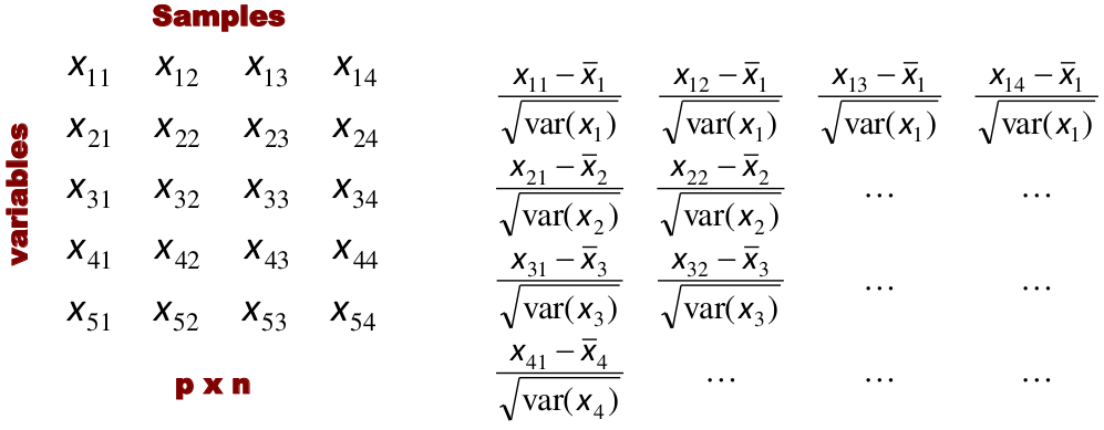
Input is data with p variables and n subjects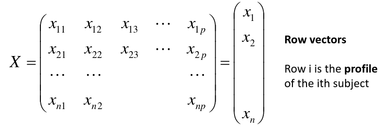

A distance between two vectors i and j must obey several rules:

The distance must be positive definite, d_ij >= 0
The distance must be symmetric, d_ij = d_ij, so that the distance from j to i is the same as the distance from i to j
An object is zero distance from itself, d_ii = 0
The triangle rule - When considering three objects i, j and k the distance from i to k is always less than or equal to the sum of the distance from i to j and the distance from j to k
d_ik <= d_ij + d_jk

Clustering Procedures

Hierarchical clustering: Iteratively merges profiles into clusters using a simple search. Start with each profile/cluster and end with one 1. The clustering procedure is represented by a dendrogram.
K-mean clustering: Start with a per-specified number of clusters and random allocation of profiles to clusters. Iteratively move profiles from one cluster to the other to optimize some criterion. End up with the same number of clusters.

K-Means Clustering

We partition the K clusters so that we maximize the similarity within clusters and minimize the similarity between clusters.

We can represent the data with a vector of means, which is the overall profile or cluster: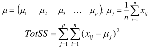

Supposed we split the data into 2 clusters, C1 with 𝑛1 observations of the p variables, and C2 with 𝑛2 observations of the p variables. We would have two different vectors of means representing the centroids of the clusters. The total sum of squares within clusters would be: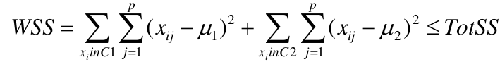

And we seek to keep WSS small, but it is NOT guaranteed to give the minimum WSS so ideally one should start from different initial values.

Start with K "random" clusters by assigning each of the n profiles to one of the K clusters at random
Iterate until no more changes are possible:
- For each of the K clusters, compute the cluster profile (centroid)
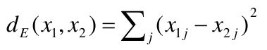
- Assign each observation to the cluster whose centroid is closest (using Euclidean distance)

Example with K = 3, p = 2: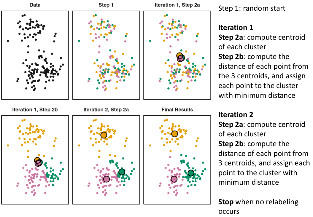

Standardization

When the variables are measured on different scales the measurement units may bias the cluster analysis. The Euclidean distance is not scale invariant.

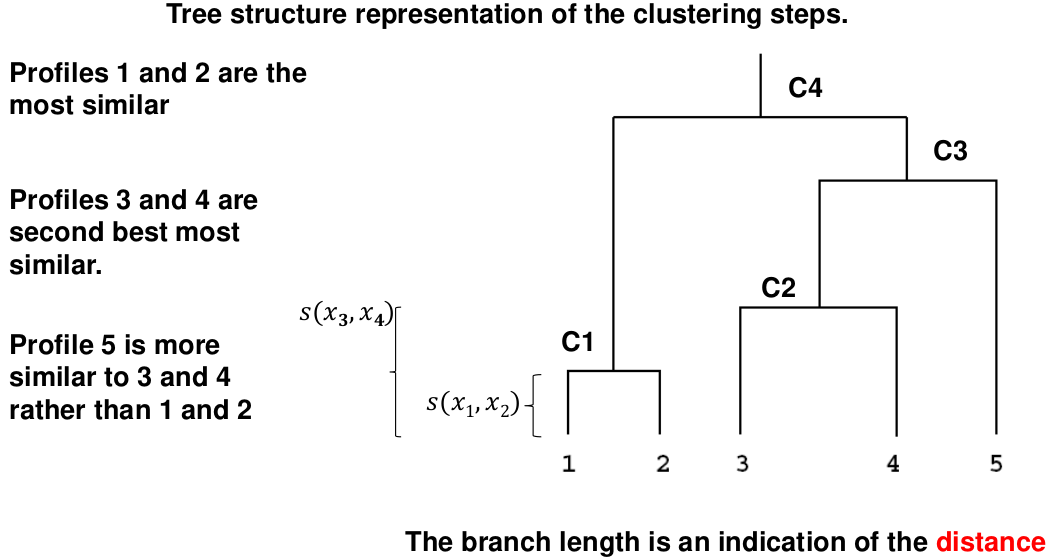
Hierarchical Clustering

This is an alternative approach that does not require a fixed number of clusters. The algorithm essentially rearranges profiles so that similar profiles are displayed next to each other in a tree (dendrogram) and the dissimilar profiles are displayed in different branches.

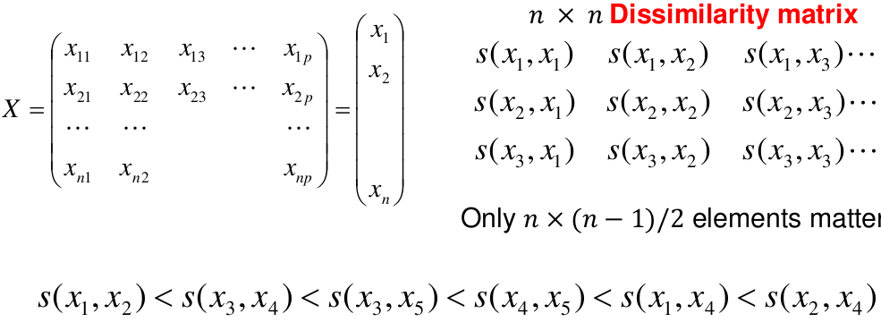
We do this we define the similarity (distance) between:

Two profiles: s(xi, xi)
A profile and a cluster: s(xc, xi)
Two clusters: s(xc, xc)

Similarity Between Clusters

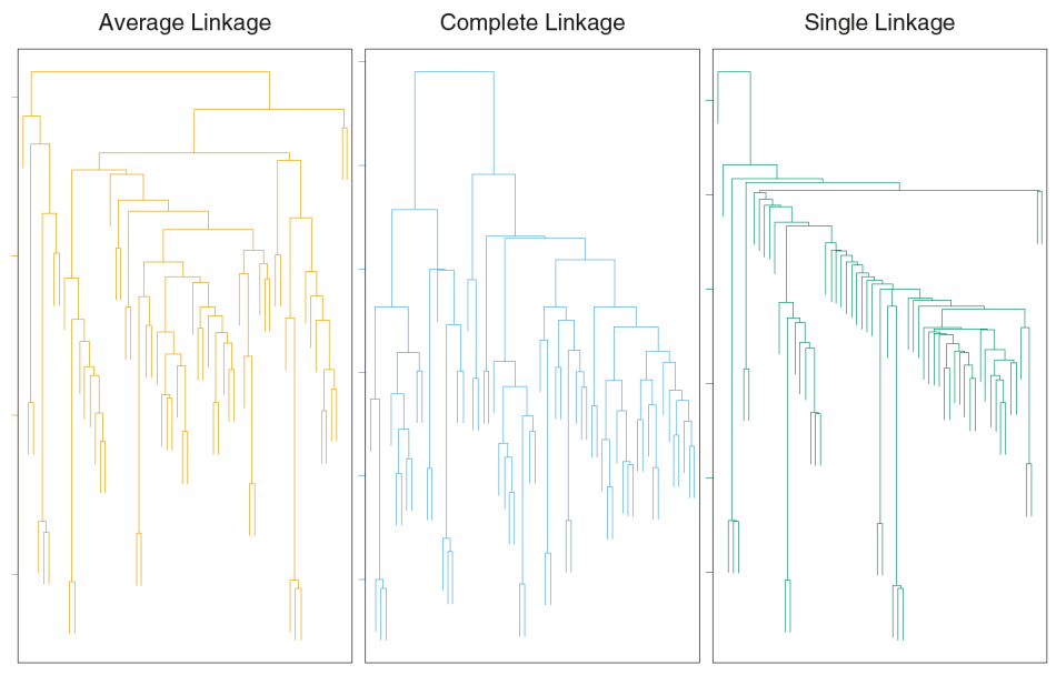
Complete-Linkage Clustering

Also known as the maximum or furthest-neighbor method
The distance between two clusters is calculated as the greatest distance between members of the relevant clusters
This method tends to produce very compact clusters of elements and the clusters are often similar in size

Single-Linkage Clustering

Referred to as the minimum or nearest neighbor method
The distance between two clusters is calculated as the minimum distance between members of the relevant clusters
This method tends to produce clusters that are 'loose' because clusters can be joined if any two members are close together. In particular, this method often results in 'chaining' or sequential addition of single samples to an existing cluster and produces trees with many long, single-addition branches.

Average-Linkage Clustering

The distance between clusters is calculated using average values. There are various methods used for calculating this average. The most common is the unweighted pair-group method average (UPGMA), where each average is calculated from the distance between each point in a cluster and all other points in another cluster and the 2 clusters with the lowest average distance are joined together into a new cluster.

Centroid Clustering

Complete and average linkage are similar, but complete linkage is faster because it does not require recalculation of the similarity matrix at each step.

Detection of Clusters

Inspection of the QQ-plot would inform about the existence of clusters in the data.

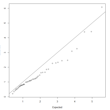
Observed and “expected” distances are statistically indistinguishable would suggest that there are no clusters in the data
Departure of the QQ-plot from the diagonal line would suggest that there are clusters

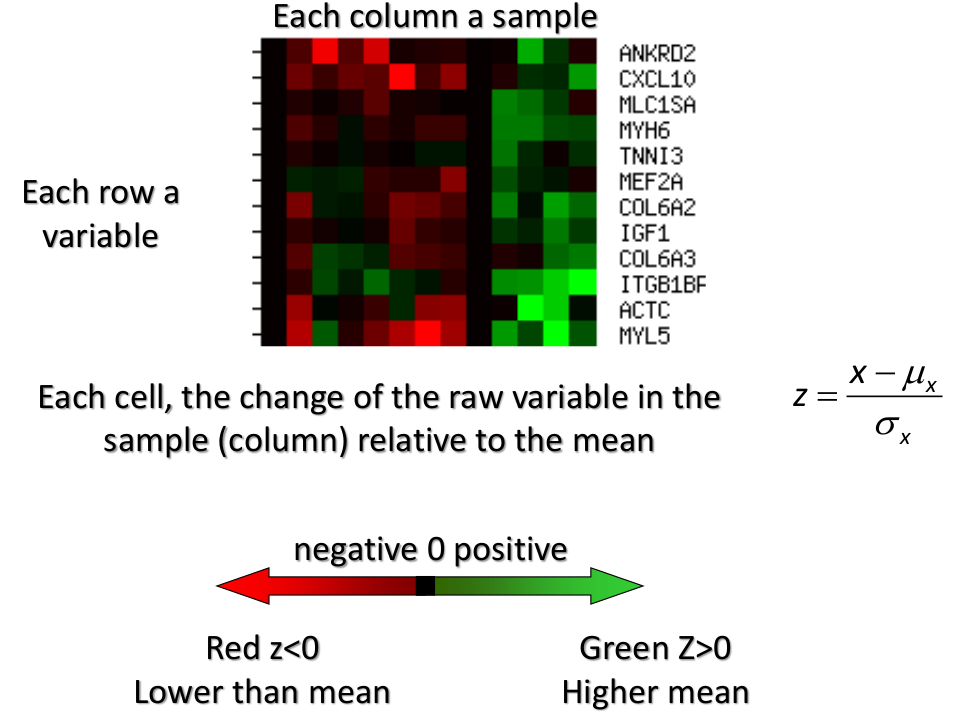
We can also use a 95%-tile to detect the number of clusters using extreme percentiles of the reference distribution. The idea is to color the entry of the data set, so that the colors represent the standardized difference of the cell intensity from a baseline. Typically, columns are samples and rows are variables.