Regression Diagnostics
The estimation and inference from the regression model depends on several assumptions. These assumptions need to be checked using regression diagnostics.
We divide the potential problems into three categories:
- Error: 𝜀 ~ N(0, 𝜎2I); i.e. the errors are:
- Independent
- Have equal variance
- Are normally distributed
- Model: The structure part of model E[y] = Xβ is correct
- Unusual observations: Sometimes just a few observations do not fit the model but might change the choice and fit of the model
Diagnostic Techniques
- Graphical
- More flexible but harder to definitively interpret
- Numerical
- Narrower in scope but require no intution
Model building is often an interactive and interactive process. It is quite common to repeat the diagnostics on a succession of models.
Unobservable Random Errors
Recall a basic multiple linear regression model is given by:
E[Y|X] = Xβ and Var(Y|X) = 𝜎2I
The vectors of errors is 𝜀 = Y - E(Y|X) = Y - Xβ; where 𝜀 is unobservable random variables with:
E(𝜀 | X) = 0
Var(𝜀 | X) = 𝜎2I
We estimate beta with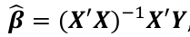
and the fitted values Y_hat corresponding to the observed value Y are: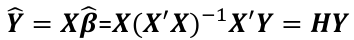
Where H is the hat matrix. Defined as: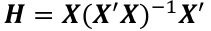
The Residuals
The vector of residuals e_hat, which can be graphed, is defined as:
E(e_hat | X) = 0
Var(e_hat | X) = 𝜎2(I - H)
Var(e_hat_i | X) = 𝜎2(I - hii); where hii is the ith diagonal element of H.
Diagnostic procedures are based on the residuals which we would like to assume behave as the unobservable errors would.
Cases with large values of hii will have small values for Var(e_hat_i | X)
The Hat Matrix
The hat matrix H is n x n symmetric matrix
- HX = X
- (I - H)X = 0
- HH = H2 = H
- Cov(Y_hat, e_hat | X) = Cov(HY, (I - H)Y| X) = 𝜎2H(I - H) = 0
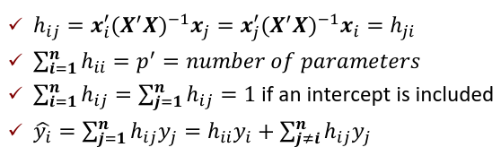
hii is also called the leverage of the ith case. As hii approaches 1, y_hat_i gets close to y_i.
Error Assumptions
We wish to check the independence, constant variance, and normality of the errors 𝜀. The errors are not observable, but we can examine the residuals e_hat.
They are NOT interchangeable with the error.
The errors may have equal variance and be uncorrelated while the residuals do not. The impact of this is usually small and diagnostics are often applied to the residuals in order to check the assumptions on the error.
Constant Variance
Check whether the variance in the residuals is related to some other quantity Y_hat and Xi
- e_hat against Y_hat: If all is well there should be constant variance in the vertical direction (e_hat) and the scatter should be symmetric vertically about 0 (linearity)
- e_hat against Xi (for predictors that are both in and out of the model): Look for the same things except in the case of plots against predictors not in the model, look for any relationship that might indicate that this predictor should be included.
- Although the interpretation of the plot may be ambiguous, one can be at least sure that nothing is seriously wrong with the assumptions.
Normality Assumptions
The tests and confidence intervals we used are based on the assumption of normal errors. The residuals can be assessed for normality using a QQ plot. This compares residuals to "ideal" normal observations.
Suppose we have a sample of n: x1, x2... xn. and wish to examine whether the x's are a sample from normal distribution:
- Order the x's to get x(1) <= x(2).... <= x(n)
- Consider a standard normal sample of size n. Let z(1) <= z(2).... <= z(n)
- If x's are normal then E[x(i)] = mean + sd*z(i); so the regression of x(i) on z(i) will be a straight line
Many statistics have been proposed for testing a sample for normality. One of these that works well is the Shapiro and Wilk W statistic, which is the square of the correlation between the observed order statistics and the expected order statistics.
- H0 is that the residuals are normal
- Only recommend this in conjunction with a QQ plot
- For a small sample size, formal tests lack power
- For a large dataset, even mild deviations from non-normality may be detected. But there would be little reason to abandon least squares because the effects of non-normality are mitigated by large sample sizes.
Testing for Curvature
One helpful test looks for curvature in the plot. Suppose we have residual e_hat vs a quantity U where U could be a regressor or a combination of regressors.
A simple test for curvature is:
- To refit the model with an additional regressor for U^2 added
- The test is based on test testing the coefficient for U^2 to be 0
- If U does not depend on estimated coefficients, then a usual t-test of this hypothesis can be used
- If U is equal to the fitted values (which depends on the estimated coefficients) then the test statistic is approximately the standard normal distribution
Unusual Observations
Some observations do not fit the model well, called outliers. Some observations change the fit of the model in a substantive manner, called influential observations. If an observation has the potential to influence the fit, it is called a leverage point.
hii is called leverage and is useful diagnostics.
Var(e_hat_i | X) = 𝜎2(1 - hii)
A large leverage will make Var(e_hat_i | X) small
The fit will be forced close to yi
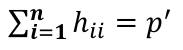 = number of parameters
An average value for hii is p'/n
A "rule of thumb": leverage > 2p'/n should be looked at more closely
hij = xi'(X'X)-1xj
Leverage only depends on X, not Y
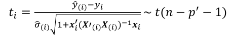
Suppose that the i-th case is suspected to be an outlier:
- We exclude point i-th case is suspected to be an outlier
- Recompute the estimates to get estimated coefficents and variance
- If y_hat_i - y_i is large, then case i is an outlier. To judge the size of potential outlier, we need to an appropriate scale:

The variance is estimated by replaced variance with estimated variance. at i - Assuming normal errors, the hypothesis E[y_hat_i - y_i] = 0 is given by


Alternative Method
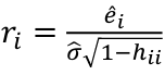
- Define standardized residual (internal studentized residual) as
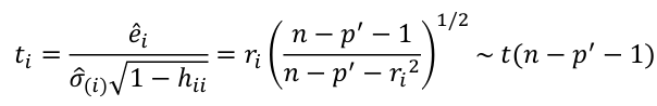
- Then studentized residual (external studentized, jackknife, or cross-validated residual, Rstudent) can be calculated as:


Bonferroni Correction
Even though we might explicitly test only one or two large ti by identifying them as large, we are implicity testing all cases. So, multiple testing correction such as Bonferroni correction should be implemented. Suppose we want a level alpha test:
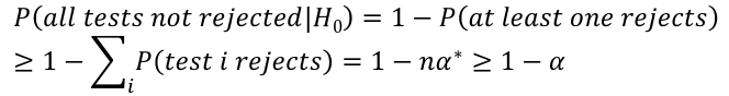
So it suggests that if an overall level alpha test is required, then a level should be alpha/n in each of the tests.
Notes on Outliers:
- An outlier in one model may not be an outlier in another when the variables have been changed or transformed
- The error distribution may not be normal and so larger residuals may be expected
- Individual outliers are usually much less of a problem in larger datasets. A single point will not have the leverage to affect the fit very much. It is still worth identifying outliers if these types of observations are worth knowing in the context.
- For large datasets, we only need to worry about clusters of outliers. Such clusters are less likely to occur by chance and more likely too represent actual structure.
When handling outliers:
- Check for a data-entry error first
- Examine the physical context, ex. the outliers in the analysis of credit card transactions may indicate fraud
- Exclude the point from the analysis but try re-including it later if the model is changed.
- Always report the existence of outliers even if they are not included in the final model!
Influential Observations
An influential point is one whose removal from the dataset causes a large change in fit. An influentual point may or may not be an outier or a leverage point.
Two meausures for identifying the infuential observations:
- Difference in Fits (DFFITS)
An observation is influential if the absolute value is greater than: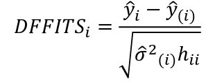
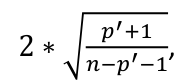 , where p is the number of parameters (predictors + 1)
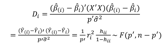
 - Cook's Distance

where p is the number of parameters (predictors + 1)- Di summarized how much alll of the fitted values change with the i-th observation is deleted
- A "rule of thumb" is Cook Distance > 4/n should be looked at more closely
- Di = 1 will potentially have important change in estimate
- Di > .5 may be influential
- Di >= 1 quite likely to be influential
- If Di sticks out from others it is almost certainly influential
- Potential Outlier's percentile value using the F-distribution ~ F(p', n-p')
- If < 10 or 20 percentile, little apparent influence
- If > 50 percentile, highly influential
- If in between, ambiguous


These rules are guidelines only, not a hard rule.
Code
## Test for normallity
gs <- lm(sqrt(Species) ~ Area + Elevation + Scruz + Nearest + Adjacent, gala)
g <- lm(Species ~ Area + Elevation + Scruz + Nearest + Adjacent, gala)

par(mfrow=c(2,2))
plot(fitted(g), residuals(g), xlab="fitted", ylab="Residuals")

qqnorm(residuals(g), ylab="Residuals")
qqline(residuals(g))

hist(g$residuals)

## Testing for curvature
library(alr4)
m2 <- lm(fertility ~ log(ppgdp) + pctUrban, UN11)
residualPlots(m2)
summary(m2)$coeff

## Testing for Outliers
g <- lm(sr ~ pop15 + pop75 + dpi + ddpi, savings)
n <- nrow(savings)
pprime <- 5   # number of parameters
jack <- rstudent(g)   # studentized residual
jack[which.max(abs(jack))]  # maximum studentized residual

# threshold for lower tail
qt(0.05/(50*2), df = n-pprime-1 , lower.tail=TRUE)

#### influential points
cook <- cooks.distance(g)
n <- nrow(savings)
pprime <- 5

check <- cook[cook > 4/n]  # rule of thumb
sort(check, decreasing=TRUE) [1:5]  # list first five max

cook[cook>0.5]    # check Di>0.5
cook[(pf(cook, pprime, n-pprime)>0.5)] # use F-dist

influenceIndexPlot(g)
No Comments