Variable Selection

Variable selection is intended to select the "best subset" of predictors. Variable selection shouldn't be separated from the rest of the model; Outliers and influential points can change the model we select. Transformations of the variables can have an impact on the model selection. Some iteration and experimentation is often necessary to find some better model.

The aim of variable selection is to construct a model that predicts or explains the relationships in the data. Automatic variable selections are not guaranteed to be consistent with these goals, so use these methods as a guide only.

The "best" subset of predictors:

Explains the data in the simplest way
Doesn't waste degrees of freedom with unnecessary predictors, which add noise
Can save time or money by not measuring redundant predictors
Doesn't include collinearity caused by too many variables trying to do the same job

There are two types of variable selections we will cover today:

Stepwise testing approach - compares successive models
The criterion approach - finds the model that optimizes some measure of goodness of fit

Model Hierarchy

Some models have a natural hierarchy, ex polynomial regression models (x² is a higher order term than x). When selecting variables it is important to respect the hierarchy. Lower order terms should not be removed from the model before higher order terms in the same variable.

Consider the model: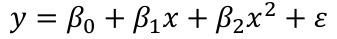

Suppose the summary shows that the term in x is not significant but x² is. If we removed x our model would become: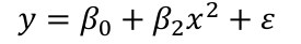

Then let's change the scale and change x to (x + a). Then the model would become:
The first order x reappears! The interpretation should not depend on the scale.

Scale changes should not make any important changes to the model.

Testing-Based Procedures

Backward Elimination

Start with all the predictors in the model
Remove the predictor with highest p-value greater than alpha
Refit the model
Remove the remaining least significant predictor provided its p-value is greater than alpha
Repeat 3 and 4 until all "non-significant" predictors are removed

Alpha is sometimes called the "p-to-remove" and does not have to be 5%. For prediction purpose, 15-20% cutoff may be best.

Forward Selection

Reverses the backwards method

Start with no variables
For predictors not in the model, check the p-value if they are added to the model. We choose the one with lowest p-value less than alpha
Continue until no new predictors can be added

Stepwise Regression

Combination of backwards elimination and forward selection.

At each stage, a variable may be added or removed and there are several variations on how this is done.
The stepwise regression can be done top-down (alternate drop step with add step) or bottom-up (alternate add step with drop step)

Notes on Testing-Based Procedures

Possible to miss the "optimal" model due to "one-at-a-time" nature of adding/dropping variables
The p-values used should not be treated too literally as there is so much multiple testing occurring
The procedures are not directly linked to final objectives of prediction or explanation
Variables that are dropped can still be correlated with the response. It is just that they provide no additional explanatory effect beyond those variables already included in the model
Stepwise selection tends to pick models smaller than desirable for prediction purpose

Criterion-Based Procedures

Criteria for model selection are based on lack of fit of a model and its complexity.

Some possible criteria:

Akaike Information Criterion (AIC):
- -2 max log-likelihood + 2p'
- n*log(RSS/n) + 2p'
Bayes Information Criterion (BIC):
- -2 max log-likelihood + p' log(n)
- n*log(RSS/n) + log(n) * p'

Note p' is the number of parameters including the intercept.

Small values of AIC and BIC are preferred. So better candidate sets will have smaller RSS and a smaller number of terms p. Larger models fit better and have smaller RSS but use more parameters. The goal is to find a balance between RSS and p.

BIC penalizes larger models more heavily. Smaller models are perferred in BIC as compared to AIC.

Adjusted R²

R² = 1 - RSS/SSY

Adding variables can only decrease RSS and increase R²
Not a good criterion as it always perfers the largest model
Important to pay attention for significant changes of RSS!

Another commonly used criterion is adjusted R², written R_a²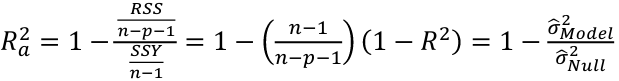

Mallow's C_p Statistics

A good model should predict well, so the average mean square error of prediction might be a good criterion: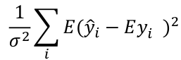
which can be estimated by the C_p statistic: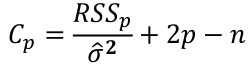

where sigma squared is from the model with ALL predictors and RSS_p indicates that RSS from a model with p parameters.

For the full model C_p = p
If a p-predictor model fits then:
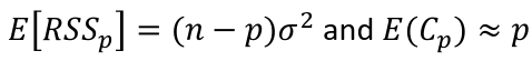
If a model has a bad fit, C_p will be much larger than p
We desire models with small p and C_p around or less than p

R Code

install.packages("faraway")
library(faraway)
data(state)
names(state)
statedata <- data.frame(state.x77, row.names=state.abb)

names(statedata)
write.csv(statedata, file="statedata.csv", quote=FALSE, row.names=F)

############# from here
## the data were collected from U.S. Bureau of the Census. 
## use life expectancy as the response
## the remaining variables as predictors

statedata <- read.csv("statedata.csv")
g <- lm(Life.Exp ~ ., data = statedata)
summary(g)

### backward elimination
g <- lm(Life.Exp ~ ., data = statedata)
summary(g)$coefficients

g <- update(g, .~ . - Area)
summary(g)$coefficients

g <- update(g, .~ . - Illiteracy)
summary(g)$coefficients

g <- update(g, .~ . - Income)
summary(g)$coefficients

g <- update(g, .~ . - Population)
summary(g)$coefficients
summary(g)

## step(lm(Life.Exp ~ ., data = statedata), 
#	scope=list(lower=as.formula(.~Illiteracy)), direction="backward")

### the variables omitted from the model may still be related to the response
summary(lm(Life.Exp ~ Illiteracy+Murder+Frost, statedata))$coeff
 
## forward
f <- ~Population + Income + Illiteracy + Murder + HS.Grad + Frost + Area
m0 <- lm(Life.Exp ~ 1, data = statedata)
m.forward <- step(m0, scope = f, direction ="forward", k=2)

## hand calculate the AIC value
aov(lm(Life.Exp ~ Murder, data=statedata))
# AIC = n*log(RSS/n) + 2p

n <- nrow(statedata)
n*log(34.46/n)+2*2

extractAIC(m.forward, k=2)		# by default k=2, AIC
extractAIC(m.forward,k=log(50))		# k=log(n), BIC

## final model using AIC
summary(m.forward)$coefficients

## use BIC
n <- nrow(statedata)
m.forward.BIC <- step(m0, scope = f, direction ="forward", 
			k=log(n), trace=FALSE)
summary(m.forward.BIC)$coefficients


### backward
m1 <- update(m0, f)
m.backward <- step(m1, scope = c(lower= ~ 1), 
			direction = "backward", trace=FALSE)
summary(m.backward)$coefficients

### stepwise
m.stepup <- step(m0, scope=f, direction="both", trace=FALSE)
summary(m.stepup)$coefficients

########## about Cp
install.packages("leaps")
library(leaps)
leaps <- regsubsets(Life.Exp ~ ., data = statedata)
rs <- summary(leaps)
par(mfrow=c(1,2))
plot(2:8, rs$cp, xlab="No. of parameters",
		ylab="Cp Statistic")
abline(0,1)

plot(2:8, rs$adjr2, xlab="No. of parameters",
		ylab="Adjusted R-Squared")
abline(0,1)
names(rs)

rs