Simple Linear Regression
One of the first known uses of regression was to study inheritance of traits from generation to generation in a study in the UK from 1893-1898. E.S. Pearson organized the collection of heights of mothers and one of their adult daughters over 18. The mother's height was the predictor variable (x) and the daughter's height was the response variable (y).
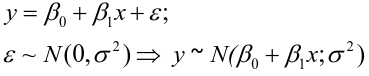
The goal of a linear regression is to quantify the relationship between one independent variable and a single dependent variable. A simple linear regression can be represented by the following:
- y_hat = β0 + β1x + Error; E(Error) = 0; V(Error) = σ2
- E(y) = β0 + β1x ; V(y) = σ2
As with correlation, a strong association in a regression analysis does NOT imply causality
Additionally, prediction values outside the range of values observed for x is not reliable, and is called extrapolation.
Least Squares Estimation
OLS/LS - Ordinary Least Squares is a method that looks for the line that minimizes the "residual sum of squares"
Residual = Observed - Predicted = y - ŷ
So we can set up an equation for sum of squared residuals: ∑(y - ŷ)2
Then substitute the linear regression equation, take the derivative, set to zero and solve.The solution comes out to:
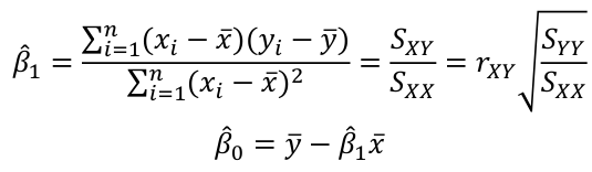
The fitted equation will pass through x bar, y bar (the center of data)
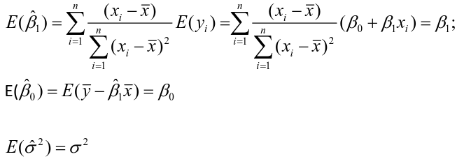
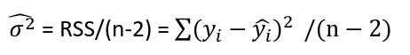
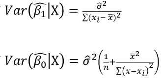
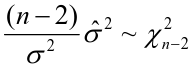
Estimating Variances of LSE
The square root of an estimated variance is called standard error represented by s or se().
E(Y |X = x) = a function that depends on the value of x
LSE Assuming Normally Distributed Data
The distributions of estimates are used to make predictions and hypothesis testing. Since variance of a fixed variable is 0, we can estimate the error of a normal distribution as follows:
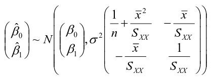
The estimates are correlated with covariance -x_bar/Sxx
It can be shown that the Least Squares Estimate is also the Maximum Likelihood Estimate.
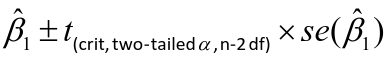
Confidence Intervals
The distribution of β1 is normal if the variance is known.
When we use estimated variance, we use a Student's t distribution on n-2 degrees of freedom to estimate parameters:
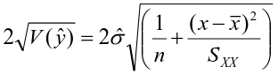
By finding the standard error of y_hat we can also calculate a confidence interval for a fitted value, or a given of x
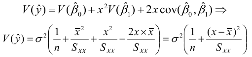
The interval width is:
And width will increase as the distance between observed and expected increases.
ANOVA
Though ANOVA is usually used in determining if there is a difference in variance with data containing 3 or more categories, linear regression under standard conditions is a special case of ANOVA. The name analysis of variance is derived from a partitioning of total variability into its component parts.
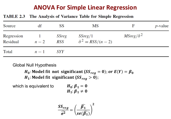
This formula uses an F-distribution with 1 and n − 2 df in place of the t-distribution to correct for the simultaneous inference from our estimate of Beta_1.
Prediction of New Observations
When using points not in the dataset (extrapolation) use the following adjusted formulas for variance of V(y):
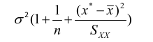
Thus, the confidence interval for a new observation would be significantly wider
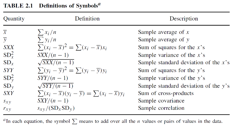
Other notations commonly seen in our textbook
No Comments