# Variable Selection
Variable selection is intended to select the "best subset" of predictors. Variable selection shouldn't be separated from the rest of the model; Outliers and influential points can change the model we select. Transformations of the variables can have an impact on the model selection. **Some iteration and experimentation is often necessary to find some better model.**
**The aim of variable selection is to construct a model that predicts or explains the relationships in the data. Automatic variable selections are not guaranteed to be consistent with these goals, so use these methods as a guide only.**
The "best" subset of predictors:
- Explains the data in the simplest way
- Doesn't waste degrees of freedom with unnecessary predictors, which add noise
- Can save time or money by not measuring redundant predictors
- Doesn't include collinearity caused by too many variables trying to do the same job
There are two types of variable selections we will cover today:
- Stepwise testing approach - compares successive models
- The criterion approach - finds the model that optimizes some measure of goodness of fit
#### Model Hierarchy
Some models have a natural hierarchy, ex polynomial regression models (x2 is a higher order term than x). When selecting variables it is important to **respect the hierarchy.** Lower order terms **should not** be removed from the model before higher order terms in the same variable.
Consider the model:
[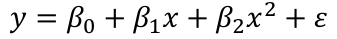](https://bookstack.mitchellhenschel.com/uploads/images/gallery/2022-10/image-1665699110928.png)
Suppose the summary shows that the term in x is not significant but x2 is. If we removed x our model would become:
[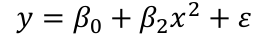](https://bookstack.mitchellhenschel.com/uploads/images/gallery/2022-10/image-1665699207039.png)
Then let's change the scale and change x to (x + a). Then the model would become:[](https://bookstack.mitchellhenschel.com/uploads/images/gallery/2022-10/image-1665699275489.png)
The first order x reappears! The interpretation should not depend on the scale.
Scale changes should not make any important changes to the model.
### Testing-Based Procedures
#### Backward Elimination
1. Start with all the predictors in the model
2. Remove the predictor with highest p-value greater than alpha
3. Refit the model
4. Remove the remaining least significant predictor provided its p-value is greater than alpha
5. Repeat 3 and 4 until all "non-significant" predictors are removed
Alpha is sometimes called the "p-to-remove" and does not have to be 5%. For prediction purpose, 15-20% cutoff may be best.
#### Forward Selection
Reverses the backwards method
1. Start with no variables
2. For predictors not in the model, check the p-value if they are added to the model. We choose the one with lowest p-value less than alpha
3. Continue until no new predictors can be added
#### Stepwise Regression
Combination of backwards elimination and forward selection.
- At each stage, a variable may be added or removed and there are several variations on how this is done.
- The stepwise regression can be done top-down (alternate drop step with add step) or bottom-up (alternate add step with drop step)
#### Notes on Testing-Based Procedures
- Possible to miss the "optimal" model due to "one-at-a-time" nature of adding/dropping variables
- The p-values used should not be treated too literally as there is so much multiple testing occurring
- The procedures are not directly linked to final objectives of prediction or explanation
- Variables that are dropped can still be correlated with the response. It is just that they provide no additional explanatory effect beyond those variables already included in the model
- Stepwise selection tends to pick models smaller than desirable for prediction purpose
### Criterion-Based Procedures
Criteria for model selection are based on lack of fit of a model and its complexity.
Some possible criteria:
- Akaike Information Criterion (AIC):
- -2 max log-likelihood + 2p'
- n\*log(RSS/n) + 2p'
- Bayes Information Criterion (BIC):
- -2 max log-likelihood + p' log(n)
- n\*log(RSS/n) + log(n) \* p'
Note p' is the number of parameters including the intercept.
**Small values of AIC and BIC are preferred.** So better candidate sets will have smaller RSS and a smaller number of terms p. Larger models fit better and have smaller RSS but use more parameters. The goal is to find a balance between RSS and p.
BIC penalizes larger models more heavily. Smaller models are perferred in BIC as compared to AIC.
#### Adjusted R2
R2 = 1 - RSS/SSY
- Adding variables can only decrease RSS and increase R2
- Not a good criterion as it always perfers the largest model
- Important to pay attention for significant changes of RSS!
Another commonly used criterion is adjusted R2, written Ra2[](https://bookstack.mitchellhenschel.com/uploads/images/gallery/2022-10/image-1665703334997.png)
#### Mallow's Cp Statistics
A good model should predict well, so the average mean square error of prediction might be a good criterion:[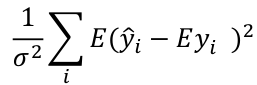](https://bookstack.mitchellhenschel.com/uploads/images/gallery/2022-10/image-1665703426676.png)
which can be estimated by the Cp statistic:
[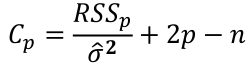](https://bookstack.mitchellhenschel.com/uploads/images/gallery/2022-10/image-1665703466451.png)
where sigma squared is from the model with ALL predictors and RSSp indicates that RSS from a model with p parameters.
- For the full model Cp = p
- If a p-predictor model fits then:
[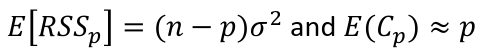](https://bookstack.mitchellhenschel.com/uploads/images/gallery/2022-10/image-1665703552755.png)
- If a model has a bad fit, Cp will be much larger than p
- **We desire models with small p and Cp around or less than p**
## R Code
```
install.packages("faraway")
library(faraway)
data(state)
names(state)
statedata <- data.frame(state.x77, row.names=state.abb)
names(statedata)
write.csv(statedata, file="statedata.csv", quote=FALSE, row.names=F)
############# from here
## the data were collected from U.S. Bureau of the Census.
## use life expectancy as the response
## the remaining variables as predictors
statedata <- read.csv("statedata.csv")
g <- lm(Life.Exp ~ ., data = statedata)
summary(g)
### backward elimination
g <- lm(Life.Exp ~ ., data = statedata)
summary(g)$coefficients
g <- update(g, .~ . - Area)
summary(g)$coefficients
g <- update(g, .~ . - Illiteracy)
summary(g)$coefficients
g <- update(g, .~ . - Income)
summary(g)$coefficients
g <- update(g, .~ . - Population)
summary(g)$coefficients
summary(g)
## step(lm(Life.Exp ~ ., data = statedata),
# scope=list(lower=as.formula(.~Illiteracy)), direction="backward")
### the variables omitted from the model may still be related to the response
summary(lm(Life.Exp ~ Illiteracy+Murder+Frost, statedata))$coeff
## forward
f <- ~Population + Income + Illiteracy + Murder + HS.Grad + Frost + Area
m0 <- lm(Life.Exp ~ 1, data = statedata)
m.forward <- step(m0, scope = f, direction ="forward", k=2)
## hand calculate the AIC value
aov(lm(Life.Exp ~ Murder, data=statedata))
# AIC = n*log(RSS/n) + 2p
n <- nrow(statedata)
n*log(34.46/n)+2*2
extractAIC(m.forward, k=2) # by default k=2, AIC
extractAIC(m.forward,k=log(50)) # k=log(n), BIC
## final model using AIC
summary(m.forward)$coefficients
## use BIC
n <- nrow(statedata)
m.forward.BIC <- step(m0, scope = f, direction ="forward",
k=log(n), trace=FALSE)
summary(m.forward.BIC)$coefficients
### backward
m1 <- update(m0, f)
m.backward <- step(m1, scope = c(lower= ~ 1),
direction = "backward", trace=FALSE)
summary(m.backward)$coefficients
### stepwise
m.stepup <- step(m0, scope=f, direction="both", trace=FALSE)
summary(m.stepup)$coefficients
########## about Cp
install.packages("leaps")
library(leaps)
leaps <- regsubsets(Life.Exp ~ ., data = statedata)
rs <- summary(leaps)
par(mfrow=c(1,2))
plot(2:8, rs$cp, xlab="No. of parameters",
ylab="Cp Statistic")
abline(0,1)
plot(2:8, rs$adjr2, xlab="No. of parameters",
ylab="Adjusted R-Squared")
abline(0,1)
names(rs)
rs
```