Module 5: Multivariate Normal Distribution
A variable X follows a discrete probability distribution if the possible values of X are either:
- A finite set
- A countable infinite sequence
px(xi) = P(X=xi) is called the probability mass function (PMF)
- px(xi) >= 0 as it is a probability
- The sum of PMF for all values of X = 1
Recall that in a Discrete Probability Distribution :
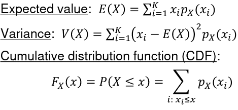
In a Continuous Probability Distribution:
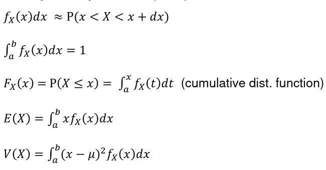
Because in a discrete set we are not concerned with the values in between our domain values.
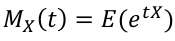
Moment Generating Function
Moments are expected values of X, such as E(X), E(X2) = E(V), E(X3), etc. This, can also be calculated using the Moment Generating Function (MGF):
The rth moment of X, E(Xr) can be obtained by differentiating Mx(t) r times with respect to t and setting t=0
- Mx(0) = 1
- MIx(0) = E(X)
- MIIx(0) = E(X2) -> V(X) = MIIx(0) - (MIx(0))2
- In general, Mx(r)(0) = E(Xr)
In short, the nth moment is the nth derivative of MGF.
Uniqueness: if X and Y are two random variables and Mx(t) = My(t) when |t| < h for some positive number h, then X and Y have the same distribution
Note: MGF does not exist for all distributions (E(etx) may be infinity)
Important Distributions
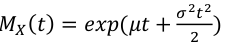
Normal Distribution
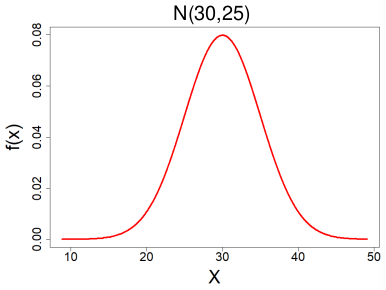
X ~ N(μ, σ2) -infinity < μ < infinity , σ < 0
- PDF:
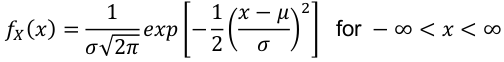
- E(X) = μ
- V(X) = σ2
- MGF:
Binomial Distribution
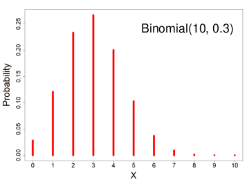
X ~ Binomial(n, p) 𝑝 ∈ [0, 1]
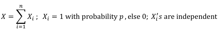
X = the number of successes in n trials when the probability of success in each trail is p.
We can think of X as the sum of n independent Bernoulli(p) random variables, with the same p for every Xi
- PMF:
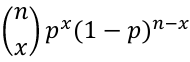
- Expected value = E(X) = np
- Variance = V(X) = np(1-p)
- MGF = Mx(t) = (pet + (1-p))n
- Two discrete random variables are independent if: P(X = x & Y = y) = P(X = x)*P(Y=y)
Ex. A study which analyzed the prevalence of a disease in a population.
Poisson Distribution
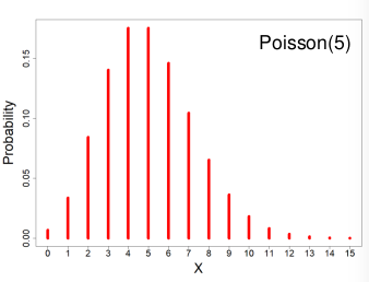
X ~ Poisson(λ) λ > 0
X = The number of occurrences of an event of interest.
- PMF:
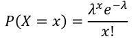
- Expected Values = E(X) = λ
- Variance = V(X) = λ
- MGF = Mx(t) = eλ(e^t - 1)
Poisson as an approximation of the Binomial Distribution
- If X ~ Binomial(n, p) and n -> infinity, p-> 0 such that np is a constant => X ~ Poisson(np)
- This assumes each event is independent
- Often used analyzing rare diseases
Ex. Analyzing lung cancer in 1000 smokers and non-smokers. This is binomial but can be estimated as a Poisson distribution.
Geometric Distribution
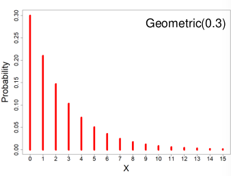
X ~ Geometric(p) 𝑝 ∈ (0, 1]
If Y1, Y2, Y3 ... are a sequence of independent Bernoulli(p) random variables then the number of failures before the first success, X, follows a Geometric distribution.
- PMF = P(X = x) = p(1-p)x
- Expected value = E(X) = (1-p)/p
- Variance = V(X) = (1-p)/p2
- MGF = Mx(t) = p / (1 - (1 - p)et)
Ex. We want to know the number of times to flip a coin before it lands on heads.
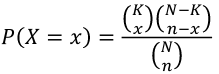
Hyper-Geometric Distribution
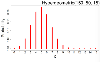
X ~ Hypergeometric(N, K, n)
Suppose a finite population of size N contains two mutually exclusive events: K success events and N-K failure events. If n events are randomly chosen without replacement X is the number of success events chosen.
- PMF:
- Expected value = E(X) = nk / N
- Variance = V(X) = ((nK) / N) * ((N-K) / N) * ((N - n) / (N - 1))
Ex. A bag has 7 red beads and 13 white beads. If 5 are drawn without replacement what is the probability exactly 4 are red?
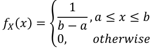
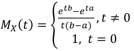
Uniform Distribution
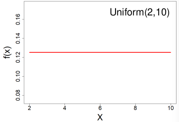
All outcomes are equally likely, they can be discrete or continuous.
X ~ Uniform(a, b) a < b
- PDF:
- E(X) = (a + b)/2
- V(X) = (b - a)2 / 12
- CDF = F(X) = (x - a) / (b -a), a<=x<=b
- MGF:
We use this distribution we use when we have no idea how the data is distributed.
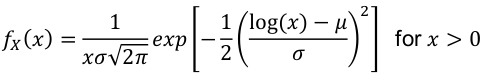
Log-Normal Distribution
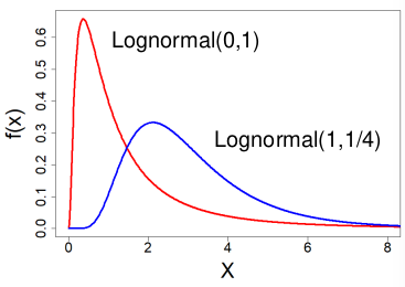
X ~ Lognormal(μ , σ2) -infinity < μ < infinity, σ > 0
- PDF:
- E(X) = exp(μ + σ2/2)
- Median = eμ
- V(X) = μ2 * (eσ^2-1)
- log(X) ~ N(μ, σ2) - the log is normal
- These distributions are often skewed to the right
Ex. Amount of rainfall, production of milk by cows, or stock market fluctuation often follow logarithmic functions.
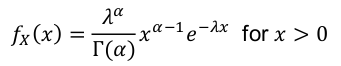
Gamma Distribution
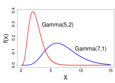
X ~ Gamma(α, λ) α > 0 , λ > 0
Used to predict the wait time until the first of event of something.
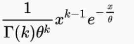
- PDF
Alternate paramterization with α > 0, 𝜃 = 1 / λ > 0 is used by R:
- E(X) = α / λ
- V(X) = α / λ2
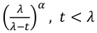
- MGF:
Ex. Used to model time to failure or time to death.
Exponential Distribution
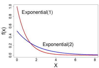
A special subset of the Gamma Distribution (α = 1)
X ~ Exponential(λ) λ > 0
- PDF = fx(x) = λ e-λ x for x > 0
- E(X) = 1 / λ
- V(X) = 1 / λ 2
- CDF = Fx(x) = 1 - e-λ x
- MGF = Mx(t) = λ / (λ - t), t < λ
Ex. The time between geyser eruptions.
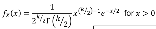
Chi-Square Distribution
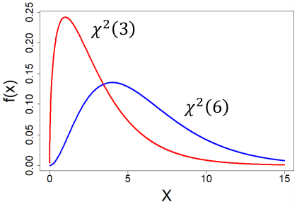
Special case of the Gamma Distribution (α = k/2, λ = 1/2)
X ~ X2(k) k is a positive integer (degrees of freedom, "df")
- PDF:
- E(X) = k
- V(X) = 2k
- MGF = (1 - 2t)-k / 2, t < 1/2
If you took a sample of Z scores and squared them you would have a chi-squared distribution with k = 1. Meaning, if Z1, Z2... Zm are independent standard normal random variables then:
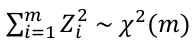
Very few real world distributions follow a chi-sqaure distribution, it is mainly used in hypothisis testing.
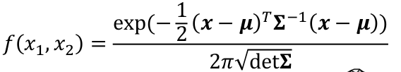
Bivariate Normal Distribution
A bivariate normal distribution is made up of two independent random variables. The two variables are both normally distributed, and have a normal distribution when added together.
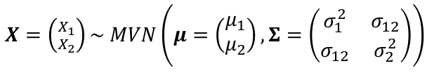
σ12 = Cov(X1, X2)
PDF:
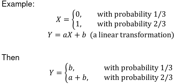
Function of a Discrete Random Variable
Suppose X is a discrete random variable and Y is a function of X. Y = g(X)
The Y is also a random variable: P(Y = y) = P(g(X) = y)
Function of a Continuous Random Variable
Using the same equation as above but assuming the variables are coninuous random variables:
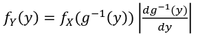
The PDF = 
The CDF = 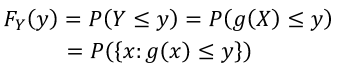
If g is one-to-one (strictly increasing or decreasing) then g has an inverse g-1, in the above case:
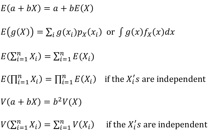
Properties of Expectation and Variance
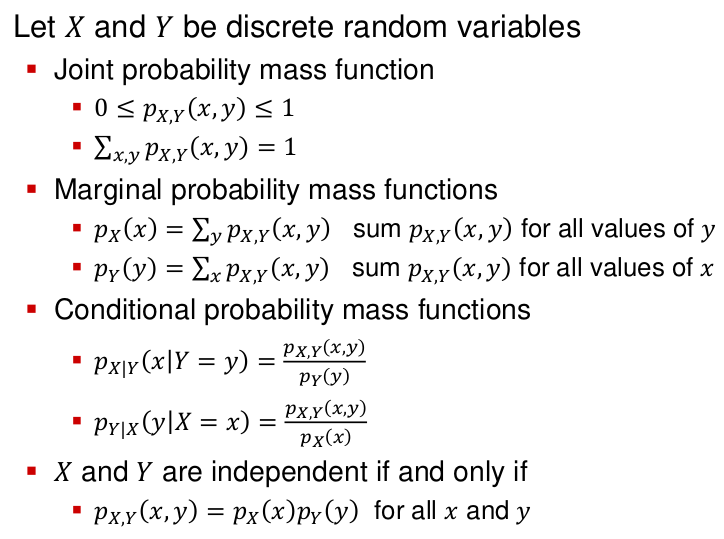
Discrete Multivariate Distributions
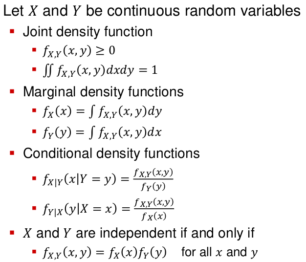
Continuous Multivariate Distributions
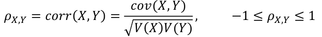
Covariance and Correlation
Correlation is defined as an indication as to how strong the relationship between the two variables is:
A positive correlation has σ > 0 and negative correlation has σ < 0
Covariance provides information about how the variables vary together:
cov(X, Y) = R[(X - E(X))(Y - E(Y))]
This is also equivalent to:
cov(X, Y) = E(XY) - E(X)*E(Y)
Thus if X and Y are independent:
cov(X, Y) = corr(X, Y) = 0
However cov(X, Y) = 0 does not imply indepence unless they are jointly normally distributed.
Conditional Expectation of X given Y = y, denoted E(X | Y = y):
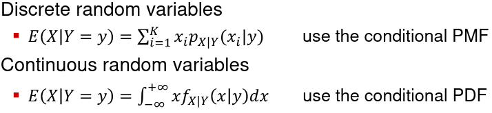
Conditional variance can be defined similarly (use the conditional PMF or PDF)
No Comments