Module 11: ANOVA - Analysis of Variance

ANOVA can be used to compare the means of several populations with continuous populations simultaneously. The population variance of the dependent variable must be equal in all groups.

Recall that 

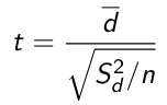
Which is the difference in two means over the standard error. When comparing multiple independent samples it is easier to use a pooled variance, but to do so the variances must be equal.

Equality of Variances

The equation for pool variance:

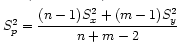
Assumption for pooled variance is that variances in the two groups are equal. We can test this with H0 = σ₁=σ₂ and use the F distribution which is indexed by the denominator df and the numerator df; choose the larger estimated variance to be numerator and the smaller estimated variance to be the denominator.

Test statistic:

If F is greater or smaller than critical values for a given significance level the null hypothesis is rejected and we can conclude there is evidence the two population variances are not equal.

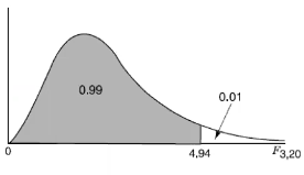
The F distribution is not symmetric, which makes it hard to look up critical values. It can be done in R: pf(F, df1, df2, lower=F)

The F test is not always appropriate as it is sensitive to departures from normality. Examine variability in the two groups by comparing sample variances using boxplots to help decide which standard error is appropriate. In the case where variances are unequal we use the same procedure but SE is estimated as:

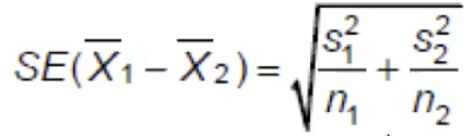
Using the n-1 degrees of freedom from whichever sample is smaller as an approximate (SAS or R would figure out the exact value).

ANOVA

Terminology:

• Factor - category/grouping variable
• Level - individual group of the factor
• Balanced design - same number of individuals in each level

The general data configuration is we have k population groups each with n_k observations, which can be the same or different.

Assumptions:

• Observations are independent
• Data are random samples from k independent populations
• Within each population the dependent variable is normally distributed
• The population variance of the dependent variable is equal in all groups.

H0: The k populations means are equal

Ha : The k populations means are not all equal or at least one is not equal

Recall that variance as a function of Y is:

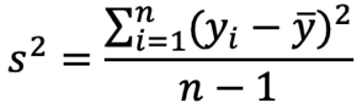
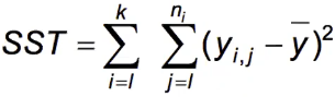
The numerator is the "Total variability" or the "Total sum of squares" (SST)

In ANOVA we split the SST into two components:

1. Variability due to differences between the groups (SS Between Groups)
2. Variability due to differences between individual y values within the groups (SS Within Group)

Which can also be expressed as:

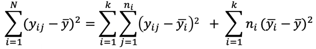
SS Total = SS Within Groups + SS Between Groups

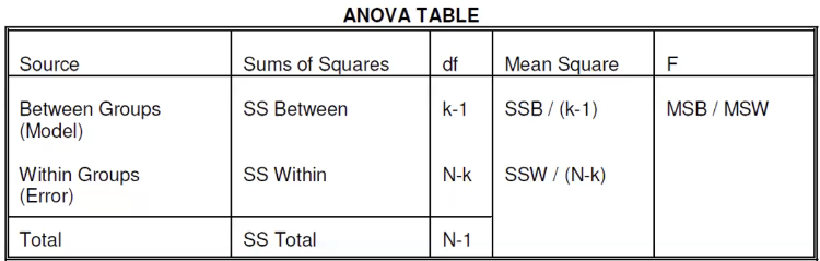
R² is the proportion of variability explained by the difference between groups:

R² = SS Between / SS Total

Adjustment Procedures

• Tukey's adjustment is appropriate when comparing pairs of means and is among the most powerful
  • Provides exact P-values when groups are equal sizes

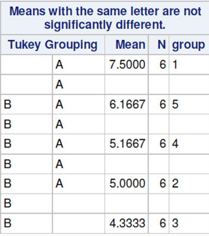
In the above Turkey procedure we observe group 1 and 3 are significantly different

• Scheffe's adjustment is appropriate for general contrasts
• Bonferroni's adjustment is appropriate for any situation but can be too conservative

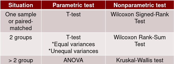
Parametric vs Non-parametric Tests

Tests are parametric because they make assumptions about the distribution of the data.

Non-parametric methods make fewer and more generic assumptions about the distribution of the data. These tests are generally more friendly toward non-normal distributions and small sample sizes.

Sign Test

Simplest non-parametric test. Analyze only the signs of the differences:

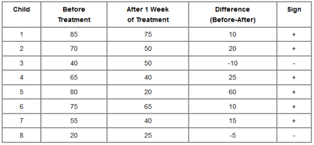
H0: The median difference is zero (half the signs are positive and half are negative)

Ha: The median difference is not zero

Wilcoxon Signed-Rank Test

Paired-sample t-test equivalent. Uses information on the relative magnitude of the paired differences as well as their signs.

Assumption:

• Independent observations
• Continuous or ordinal observations
• Symmetric distribution

H0: The median difference is zero

Ha: The median difference is not zero

1. Rank the magnitude of the differences (ignoring the signs)
2. Attach the signs to the ranks to form signed ranks
3. Calculate the test statistic, R, which is the sum of the positive ranks.
4. n≥20 → normal approximation
 The values of the test statistic will range from 0 to N(N+1)/2, with a mean value of N(N+1)/4

Wilcoxon Rank-Sum Test

For two independent samples

Assumption:

• Independent observations
• Continuous or ordinal observations
  
• If using as a test of median, samples must have the same shape

H0: Distributions of populations from which the two groups are samples are the same.

Ha: Distributions of populations from which the two groups are samples are not the same.

1. Combine the two groups into one large sample and rank the observations from smallest to largest. Tied observations are assigned a average rank to all measurements with the same value.
2. Sum the ranks of each of the original groups.
3. The Wilcoxon sum rank test statistic (R) is the sum of the ranks in the group with the smallest sum

Kruskal-Wallis Test

A non-parametric analogue to one-way ANOVA. It's an extension of the Wilcoxon rank-sum test for more than two groups. Based on ranked data. The Kruskal Wallis test will tell you if there is a significant difference between groups. However, it won’t tell you which groups are different.

Assumption:

• Use when normality assumption is violated.
  
• Samples drawn from population are random
• Observations are independent
• The dependent variable is at least ordinal
• All groups have the same distribution shape

H0: The population medians are equal in all groups

Ha: At least one of the groups population median is different

Step 1: Rank data without respect to group (rank the data from 1 to N ignoring group membership).
rij = rank of yij
Tie values obtain the rank of the average rank they would receive if not tied
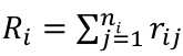
Step 2: For each group i, compute 

Step 3: Calculate h*

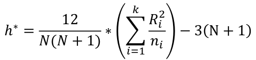
When H0 is true, h* has an approximate chi-square distribution with k-1 degrees of freedom

When we have tied values, need to make additional adjustments to h.

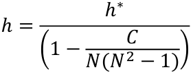
If g is the categories of tied values, the Lth category can be described as c_L = m * (m² - 1), where m is the number of ties values for the Lth category. The correction factor is C = c1 + c2 + ... + cg