Module 13: Linear Regression

Correlation and regression attempt to describe the strength and direction of the association between two (or more) continuous variables.

Pearson Correlation

Recall r is an estimate of population correlation coefficient:

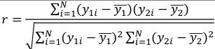
It is always between -1 and 1. With 0 indicating no positive or negative linear relationship between the variables.

A strong correlation does not imply causality.

It indicates the strength and direction of a linear relationship between two random variables. The square of r, r² = R,  measures how much information is shared between two variables; It is also called the coefficient of determination.

R² can be explained as the proportion of the variability in y that can be explained by the independent variables (X).

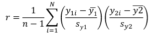
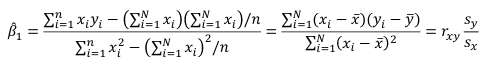
r can also be expressed as the average product in standard units in terms of sample standard deviations:

Assumptions for Pearson's Correlation:

• Observations are independent
• The association is linear
• Variables are approximately normally distributed

We can compute a test statistic for r with a t-distribution:

t = r / se(r);  Where SE of r = sqrt((1-r^2)/(n-2))

Note that se is inversely related to n, so a large sample size results in a smaller se(r). Also the test has n-2 degrees of freedom.

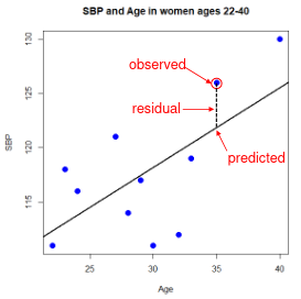
Simple Linear Regression

Linear regression is used to quantify the relationship between one or more independent variables (X) and a single dependent variables (Y). Simple linear regression is the case when we have 1 independent continuous variable and 1 dependent continuous variable.

The line of best fit is the line which minimized  the least squares (LS) estimate:

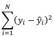
The sum of predicted minus observed values squared. For regressions with only one independent variable, X, this yields to the following equation:

 

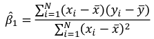
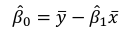
We can take the derivative with respect to each beta and set equal to 0 to end up with the following 2 equations:

Even after we find our best fit line, we cannot predict values that were outside of our sample range.

Estimated Variances of Estimates

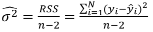
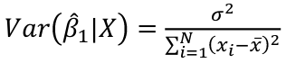
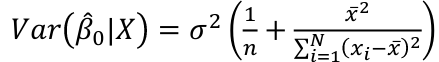
The square root of estimated variance is Standard Error (SE).

In R, the lm() function can be used to determine the simple linear regression:

res <-  lm(var_y ~ var_x, data=mydata)

Sum of Squares

Model SS - SS of the differences between y predicted by the model and the overall average. (y_hat - y_bar)^2

Error SS - SS of the differences between y observed and the y predicted by the model. (yi - y_hat)^2

Total SS - SS of the differences between y observed by the model and the overall average. (yi - y_bar)^2

The better the model fits the larger the model SS and the smaller the Error SS.

F Values

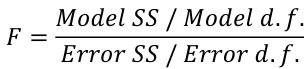
The numerator df is for the model and the denominator df is for error. In a situation with one 1 X variable, the F-test is equivalent to the t-test for the null hypothesis that β₁ =0.

Also notice that in the case of one predictor, F is the square of t.