Module 8: Interval Estimation

• θ is fixed while θ_{hat_n} is a random variable which provides the single best value to estimate θ
  
• θ_hat is unbiased when bias = E(θ_{hat_n) -} θ = 0
  
• θ_hat is consistent when θ_{hat_n ->} θ
• Mean squared error MSE = E(θ_{hat_n -} θ)² = bias(θ_{hat_n}) + V(θ_{hat_n})
• If bias -> and se -> as n -> infinity then θ_{hat_n} is consistent
  
• Probability is stronger than samples, probability standard error eventually converges to 0 as n approaches infinity but samples converge to a normal distribution which is not necessarily the same as the population distribution.
• We the estimator variability (se) to provide an interval of parameter values that are "supported" by the sample.

A 1 - α confidence interval for a parameter θ is an interval C_n = (a; b) where a = a(X₁, ...X_n) and b = b(X₁, ...X_n) are functions of the data such that:  P(θ ∈ C_n) >= 1 - α   ; Where θ is the actual population mean. C_n is random and θ is fixed.

The confidence interval (a; b) capture the true mean with confidence 1 - α. We commonly use 95% confidence intervals which corresponds to α = .05. This does NOT mean there is 1- α chance/probability the parameter falls in the interval. The correct interpretation: If we repeatedly take samples of size n from a fixed and stable population and build a 95% confidence intervals, 95% of these intervals would contain the true unknown parameter.

CI For Mean of a Normal Distribution

If σ² is known:  X_bar +/- Z_α/2*α_x

If σ² is unknown:  X_bar +/- t_(α/2,n-1)*S/sqrt(n); Where S² = 1/(n-1) * sum(x_i-x_bar)²

Using S in place of SD causes more uncertainty, thus increasing the size of the CI.

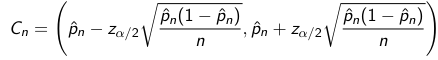
We can similarly find the confidence interval of a proportion in a similar manner:

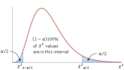
Chi-Square DIstribution

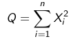
The above represents the chi-squared distribution with n degrees of freedom. E(Q) = n and V(Q) = 2n.

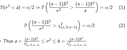
The distribution of X²_n-1 is not symmetrical, so instead of centering our CI (a,b) on the mean, we look for symmetry so that the bounds P(θ < a) = α/2 and P(θ > b) = α/2.

We derive the variance of a distribution through Fisher's theorem (not shown). The CI comes out to:

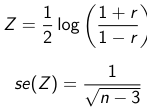
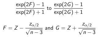
Pearson's product Moment Correlation Coefficient is between -1 and 1 and represents the correlation between 2 variables.

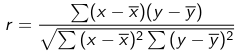
Although rarely used, you could find a confidence interval for this value.