# Module 5: Multivariate Normal Distribution
A variable X follows a discrete probability distribution if the possible values of X are either:
- A finite set
- A countable infinite sequence
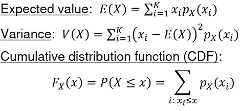
px(xi) = P(X=xi) is called the probability mass function (PMF)
- px(xi) >= 0 as it is a probability
- The sum of PMF for all values of X = 1
Recall that in a Discrete Probability Distribution :
[](https://bookstack.mitchellhenschel.com/uploads/images/gallery/2022-08/image-1660918683481.png)
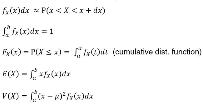
In a Continuous Probability Distribution:
[](https://bookstack.mitchellhenschel.com/uploads/images/gallery/2022-08/image-1660918718518.png)
Because in a discrete set we are not concerned with the values in between our domain values.
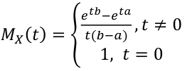
### Moment Generating Function
Moments are expected values of X, such as E(X), E(X2) = E(V), E(X3), etc. This, can also be calculated using the Moment Generating Function (MGF):
[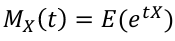](https://bookstack.mitchellhenschel.com/uploads/images/gallery/2022-08/image-1660918098650.png)
The rth moment of X, E(Xr) can be obtained by differentiating Mx(t) r times with respect to t and setting t=0
- Mx(0) = 1
- MIx(0) = E(X)
- MIIx(0) = E(X2) -> V(X) = MIIx(0) - (MIx(0))2
- In general, Mx(r)(0) = E(Xr)
In short, the nth moment is the nth derivative of MGF.
Uniqueness: if X and Y are two random variables and Mx(t) = My(t) when |t| < h for some positive number h, then X and Y have the same distribution
Note: MGF does not exist for all distributions (E(etx) may be infinity)
## Important Distributions
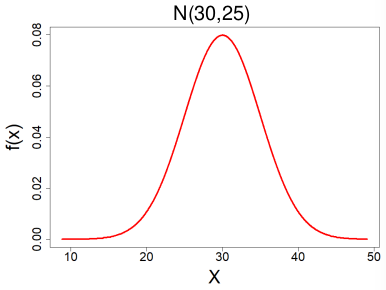
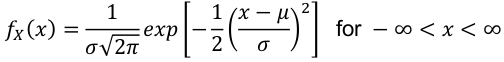
#### Normal Distribution
[](https://bookstack.mitchellhenschel.com/uploads/images/gallery/2022-08/image-1661008157874.png)
X ~ N(μ, σ2) -infinity < μ < infinity , σ < 0
- PDF:
[](https://bookstack.mitchellhenschel.com/uploads/images/gallery/2022-08/image-1661008301108.png)
- E(X) = μ
- V(X) = σ2
- MGF:
[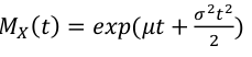](https://bookstack.mitchellhenschel.com/uploads/images/gallery/2022-08/image-1661008355636.png)
#### Binomial Distribution
[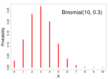](https://bookstack.mitchellhenschel.com/uploads/images/gallery/2022-08/image-1661007837488.png)
X ~ Binomial(n, p) 𝑝 ∈ \[0, 1\]
X = the number of successes in n trials when the probability of success in each trail is p.
We can think of X as the sum of n independent Bernoulli(p) random variables, with the same p for every Xi
[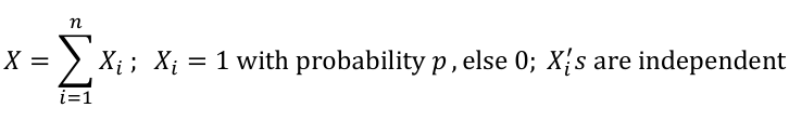](https://bookstack.mitchellhenschel.com/uploads/images/gallery/2022-08/image-1660920861915.png)
- PMF:
[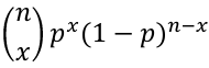](https://bookstack.mitchellhenschel.com/uploads/images/gallery/2022-08/image-1660918544947.png)
- Expected value = E(X) = np
- Variance = V(X) = np(1-p)
- MGF = Mx(t) = (pet + (1-p))n
- Two discrete random variables are independent if: P(X = x & Y = y) = P(X = x)\*P(Y=y)
Ex. A study which analyzed the prevalence of a disease in a population.
#### Poisson Distribution
[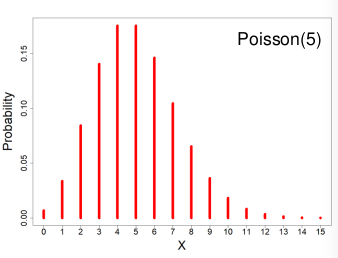](https://bookstack.mitchellhenschel.com/uploads/images/gallery/2022-08/image-1661008056947.png)
X ~ Poisson(λ) λ > 0
X = The number of occurrences of an event of interest.
- PMF:
[](https://bookstack.mitchellhenschel.com/uploads/images/gallery/2022-08/image-1660920679945.png)
- Expected Values = E(X) = λ
- Variance = V(X) = λ
- MGF = Mx(t) = eλ(e^t - 1)
Poisson as an approximation of the Binomial Distribution
- If X ~ Binomial(n, p) and n -> infinity, p-> 0 such that np is a constant => X ~ Poisson(np)
- This assumes each event is independent
- Often used analyzing rare diseases
Ex. Analyzing lung cancer in 1000 smokers and non-smokers. This is binomial but can be estimated as a Poisson distribution.
#### Geometric Distribution
[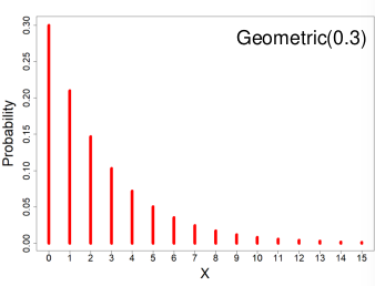](https://bookstack.mitchellhenschel.com/uploads/images/gallery/2022-08/image-1661008075865.png)
X ~ Geometric(p) 𝑝 ∈ (0, 1\]
If Y1, Y2, Y3 ... are a sequence of independent Bernoulli(p) random variables then the number of failures before the first success, X, follows a Geometric distribution.
- PMF = P(X = x) = p(1-p)x
- Expected value = E(X) = (1-p)/p
- Variance = V(X) = (1-p)/p2
- MGF = Mx(t) = p / (1 - (1 - p)et)
Ex. We want to know the number of times to flip a coin before it lands on heads.
#### Hyper-Geometric Distribution
[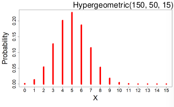](https://bookstack.mitchellhenschel.com/uploads/images/gallery/2022-08/image-1661008089863.png)
X ~ Hypergeometric(N, K, n)
Suppose a finite population of size N contains two mutually exclusive events: K success events and N-K failure events. If n events are randomly chosen *without* replacement X is the number of success events chosen.
- PMF:
[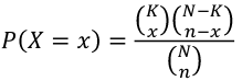](https://bookstack.mitchellhenschel.com/uploads/images/gallery/2022-08/image-1660921389776.png)
- Expected value = E(X) = nk / N
- Variance = V(X) = ((nK) / N) \* ((N-K) / N) \* ((N - n) / (N - 1))
Ex. A bag has 7 red beads and 13 white beads. If 5 are drawn *without* replacement what is the probability exactly 4 are red?
#### Uniform Distribution
[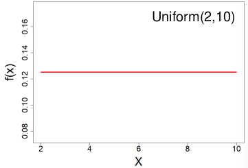](https://bookstack.mitchellhenschel.com/uploads/images/gallery/2022-08/image-1661008106329.png)
All outcomes are equally likely, they can be discrete or continuous.
X ~ Uniform(a, b) a < b
- PDF:
[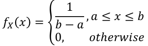](https://bookstack.mitchellhenschel.com/uploads/images/gallery/2022-08/image-1660922154972.png)
- E(X) = (a + b)/2
- V(X) = (b - a)2 / 12
- CDF = F(X) = (x - a) / (b -a), a<=x<=b
- MGF:
[](https://bookstack.mitchellhenschel.com/uploads/images/gallery/2022-08/image-1660922288816.png)
We use this distribution we use when we have no idea how the data is distributed.
#### Log-Normal Distribution
[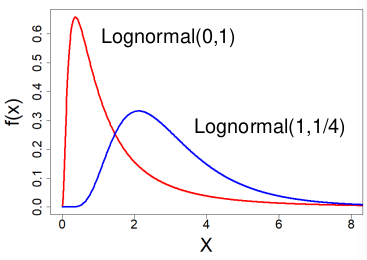](https://bookstack.mitchellhenschel.com/uploads/images/gallery/2022-08/image-1661008395275.png)
X ~ Lognormal(μ , σ2) -infinity < μ < infinity, σ > 0
- PDF:
[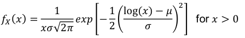](https://bookstack.mitchellhenschel.com/uploads/images/gallery/2022-08/image-1661008422821.png)
- E(X) = exp(μ + σ2/2)
- Median = eμ
- V(X) = μ2 \* (eσ^2-1)
- log(X) ~ N(μ, σ2) - the log is normal
- These distributions are often skewed to the right
Ex. Amount of rainfall, production of milk by cows, or stock market fluctuation often follow logarithmic functions.
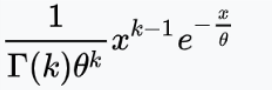
#### Gamma Distribution
[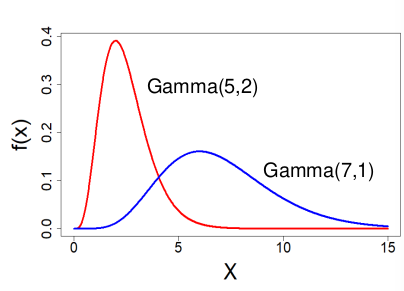](https://bookstack.mitchellhenschel.com/uploads/images/gallery/2022-08/image-1661008814686.png)
X ~ Gamma(α, λ) α > 0 , λ > 0
Used to predict the wait time until the first of event of something.
- PDF
[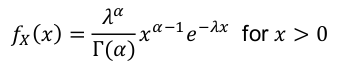](https://bookstack.mitchellhenschel.com/uploads/images/gallery/2022-08/image-1661008839904.png)
Alternate paramterization with α > 0, 𝜃 = 1 / λ > 0 is used by R:
[](https://bookstack.mitchellhenschel.com/uploads/images/gallery/2022-08/image-1661009165290.png)
- E(X) = α / λ
- V(X) = α / λ2
- MGF:
[](https://bookstack.mitchellhenschel.com/uploads/images/gallery/2022-08/image-1661008903685.png)
Ex. Used to model time to failure or time to death.
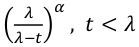
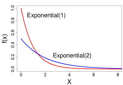
#### Exponential Distribution
[](https://bookstack.mitchellhenschel.com/uploads/images/gallery/2022-08/image-1661009476997.png)
A special subset of the Gamma Distribution (α = 1)
X ~ Exponential(λ) λ > 0
- PDF = fx(x) = λ e-λ x for x > 0
- E(X) = 1 / λ
- V(X) = 1 / λ 2
- CDF = Fx(x) = 1 - e-λ x
- MGF = Mx(t) = λ / (λ - t), t < λ
Ex. The time between geyser eruptions.
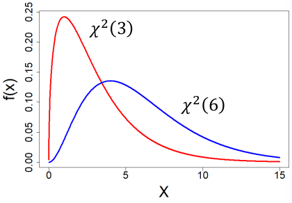
#### Chi-Square Distribution
[](https://bookstack.mitchellhenschel.com/uploads/images/gallery/2022-08/image-1661009672800.png)
Special case of the Gamma Distribution (α = k/2, λ = 1/2)
X ~ *X*2(k) k is a positive integer (degrees of freedom, "df")
- PDF:
[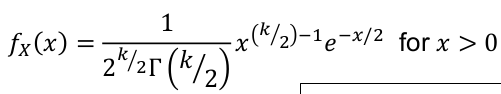](https://bookstack.mitchellhenschel.com/uploads/images/gallery/2022-08/image-1661009613379.png)
- E(X) = k
- V(X) = 2k
- MGF = (1 - 2t)-k / 2, t < 1/2
If you took a sample of Z scores and squared them you would have a chi-squared distribution with k = 1. Meaning, if Z1, Z2... Zm are independent standard normal random variables then:
[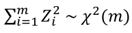](https://bookstack.mitchellhenschel.com/uploads/images/gallery/2022-08/image-1661009823858.png)
Very few real world distributions follow a chi-sqaure distribution, it is mainly used in hypothisis testing.
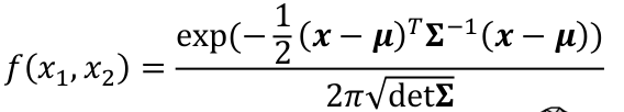
#### Bivariate Normal Distribution
A bivariate normal distribution is made up of two independent random variables. The two variables are both normally distributed, and have a normal distribution when added together.
[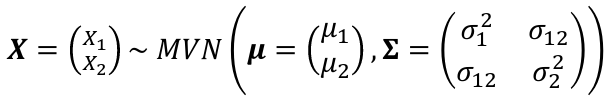](https://bookstack.mitchellhenschel.com/uploads/images/gallery/2022-08/image-1660924679433.png)
σ12 = Cov(X1, X2)
PDF:
[](https://bookstack.mitchellhenschel.com/uploads/images/gallery/2022-08/image-1661012030416.png)
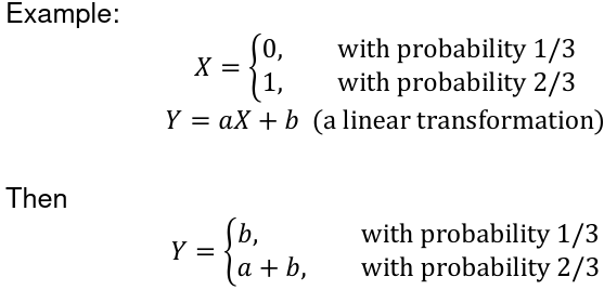
#### Function of a Discrete Random Variable
Suppose X is a discrete random variable and Y is a function of X. Y = g(X)
The Y is also a random variable: P(Y = y) = P(g(X) = y)
[](https://bookstack.mitchellhenschel.com/uploads/images/gallery/2022-08/image-1660923222954.png)
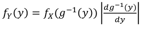
#### Function of a Continuous Random Variable
Using the same equation as above but assuming the variables are coninuous random variables:
The PDF = [](https://bookstack.mitchellhenschel.com/uploads/images/gallery/2022-08/image-1660923084277.png)
The CDF = [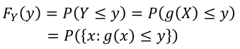](https://bookstack.mitchellhenschel.com/uploads/images/gallery/2022-08/image-1660923112070.png)
If g is one-to-one (strictly increasing or decreasing) then g has an inverse g-1, in the above case:
[](https://bookstack.mitchellhenschel.com/uploads/images/gallery/2022-08/image-1660923301389.png)
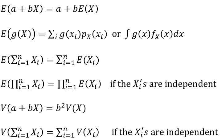
### Properties of Expectation and Variance
[](https://bookstack.mitchellhenschel.com/uploads/images/gallery/2022-08/image-1661010254301.png)
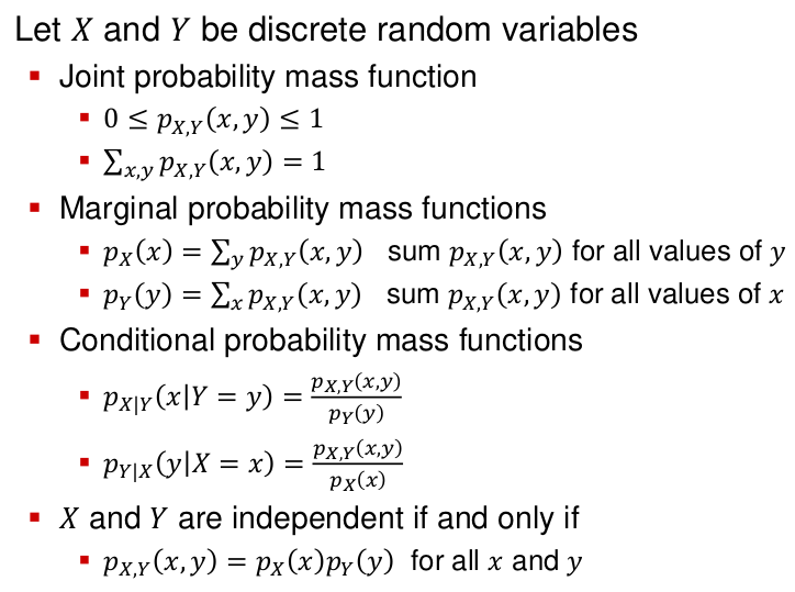
### Discrete Multivariate Distributions
[](https://bookstack.mitchellhenschel.com/uploads/images/gallery/2022-08/image-1661010303330.png)
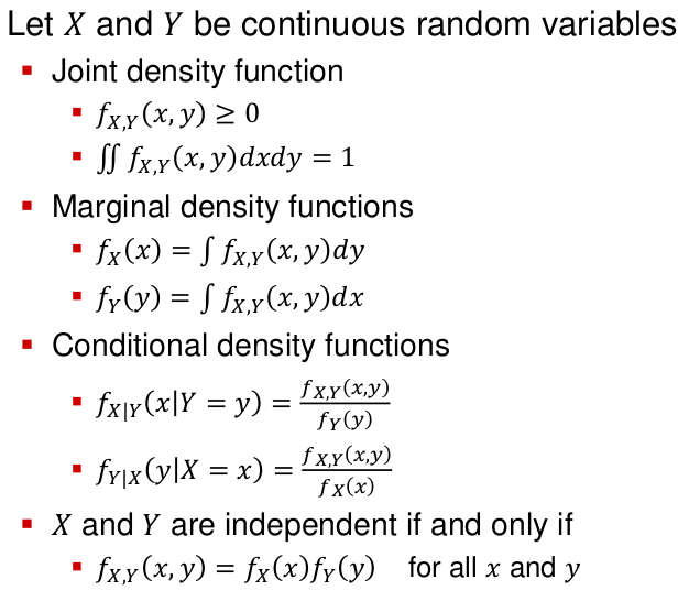
### Continuous Multivariate Distributions
[](https://bookstack.mitchellhenschel.com/uploads/images/gallery/2022-08/image-1661010356599.png)
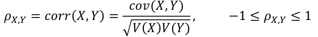
### Covariance and Correlation
**Correlation** is defined as an indication as to how strong the relationship between the two variables is:
[](https://bookstack.mitchellhenschel.com/uploads/images/gallery/2022-08/image-1660924208472.png)
A positive correlation has σ > 0 and negative correlation has σ < 0
**Covariance** provides information about how the variables vary together:
cov(X, Y) = R\[(X - E(X))(Y - E(Y))\]
This is also equivalent to:
cov(X, Y) = E(XY) - E(X)\*E(Y)
Thus if X and Y are independent:
cov(X, Y) = corr(X, Y) = 0
However cov(X, Y) = 0 does not imply indepence unless they are jointly normally distributed.
**Conditional Expectation** of X given Y = y, denoted E(X | Y = y):
[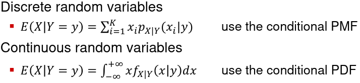](https://bookstack.mitchellhenschel.com/uploads/images/gallery/2022-08/image-1660924494462.png)
**Conditional variance** can be defined similarly (use the conditional PMF or PDF)