Module 3: Random Variables and Normal Distributions
A variable is a measurement or characteristic on which individual observations are made. A random variable is a variable whose possible values are outcomes of a random phenomenon. A domain is a set of all possible values a variable can take.
Discrete random variables is a finite set or countably infinite sequence.
px(xi) = P(X = xI) is called the Probability Mass Function (PMF).
- 0 <= px(xi) <= 1 as it is a probability,
- Sum of PMF for all values of X = 1.
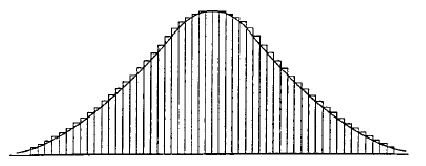
Continuous random variable can lie on a numerical scale, such as all real numbers between (0, +infinity). If we mapped the data to a histogram, we would see the curve begin to smooth as the number of data points approaches infinity.
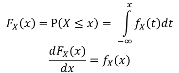
This density curve, fx(x), is called the Probability Density Function (PDF).
- fx(x) >= 0 but can be greater than 1
- The integral of fx(x) over the domain of X is 1
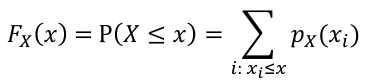
The Cumulative Distribution Function (CDF) is defined as Fx(X) = P(X <= x)
- Non-decreasing
- The limit toward -infinity is 0, toward +infinity is 1
- For discrete random variables:
- For continuous random variables:
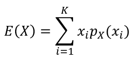
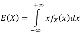
The Expected Value of a random variable is an average of the possible values weighted by their probabilities. Also called mean and denoted by μ.
- For discrete random variables
- For continuous random variables
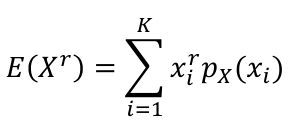
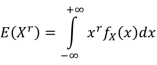
A generalization for the expected values is the rth moment of a random variables, R(Xr).
- For discrete random variables:
- For continuous random variables:
The first moment of a random variable is the expect value (mean). The rth moment of a random variable about the mean, also called the rth central moment, is defined as: E[(X - μ)r]
- The first central moment = 0
- The second central moment is the variance denoted as 𝜎2
The variance measures the spread around the mean of a random variable: Var(X) = E[(X - μ)2]
- Also equivelent to Var(X) = E(X2) - [E(X)]2
- The standard deviation is the square root of the variance
The normal distribution:
- is a continuous distribution
- can be expressed by a formula
- also called Gaussian distribution
- is a theoretical model for a population distribution that approximates the distribution of a number of measurement variables
- is appropriate for a number of measures, but not all. Only appropriate for some continuous measurements.
- is symmetric about the mean (i.e P(X > μ) = P(X < μ) = .5)
- is completely characterized mean and variance
The 68/95/99 rule:
- 68.25% of the data falls within 1 SD
- 95.45% of the data falls within 2 SD
- 99.74% of the data falls within 3SD
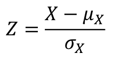
The standard normal random variable, referred to as Z, is in the scale of SD units from the mean.
Z has a μ=0 and SD = 1 we can standardize any normal distribution with:
By converting to Z-scores we can easily compare the probability events in two different normal distribution.
The kth percentile is defined as the score that holds the k percent of the scores below it. Ex. 90th percentile is the score that has 90% of the scores below it. We can compute percentiles with: X = μ + Z𝜎
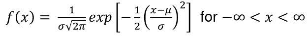
The probability density function for normal curves:
And in normal curves when mean is 0 and SD is 1 this can be simplified.
Relevant R Functions
qnorm(percentile, μ, 𝜎) computes percentiles for normal variables
dnorm(x, μ, 𝜎) will return the height of normal density function with a certain mean and SD at point x
pnorm(z, μ, 𝜎) will return the cumulative distribution function of a normal distribution with certain mean and SD
No Comments