A strong correlation does not imply causality.
It indicates the strength and direction of a linear relationship between two random variables. The square of r, r2 = R, measures how much information is shared between two variables; It is also called the coefficient of determination.R2 can be explained as the proportion of the variability in y that can be explained by the independent variables (X).
r can also be expressed as the average product in standard units in terms of sample standard deviations: [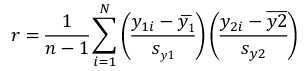](https://bookstack.mitchellhenschel.com/uploads/images/gallery/2022-08/image-1661955971008.png) Assumptions for Pearson's Correlation: - Observations are independent - The association is linear - Variables are approximately normally distributed We can compute a test statistic for r with a t-distribution: t = r / se(r); Where SE of r = sqrt((1-r^2)/(n-2)) Note that se is inversely related to n, so a large sample size results in a smaller se(r). Also the test has n-2 degrees of freedom. ### Simple Linear Regression Linear regression is used to quantify the relationship between one or more independent variables (X) and a single dependent variables (Y). Simple linear regression is the case when we have 1 independent continuous variable and 1 dependent continuous variable. [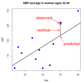](https://bookstack.mitchellhenschel.com/uploads/images/gallery/2022-08/image-1661958084862.png) The line of best fit is the line which minimized the least squares (LS) estimate: [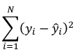](https://bookstack.mitchellhenschel.com/uploads/images/gallery/2022-08/image-1661958510054.png) The sum of predicted minus observed values squared. For regressions with only one independent variable, X, this yields to the following equation: [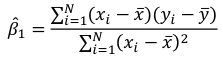](https://bookstack.mitchellhenschel.com/uploads/images/gallery/2022-08/image-1661958589368.png) We can take the derivative with respect to each beta and set equal to 0 to end up with the following 2 equations: [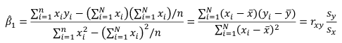](https://bookstack.mitchellhenschel.com/uploads/images/gallery/2022-08/image-1661966730576.png) [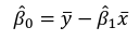](https://bookstack.mitchellhenschel.com/uploads/images/gallery/2022-08/image-1661958600629.png) Even after we find our best fit line, we cannot predict values that were outside of our sample range. #### Estimated Variances of Estimates [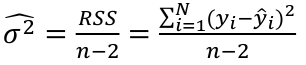](https://bookstack.mitchellhenschel.com/uploads/images/gallery/2022-08/image-1661959107275.png) [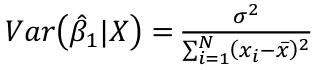](https://bookstack.mitchellhenschel.com/uploads/images/gallery/2022-08/image-1661959120502.png) [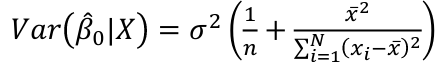](https://bookstack.mitchellhenschel.com/uploads/images/gallery/2022-08/image-1661959136704.png) The square root of estimated variance is Standard Error (SE). In R, the lm() function can be used to determine the simple linear regression: > res <- lm(var\_y ~ var\_x, data=mydata) #### Sum of Squares Model SS - SS of the differences between y predicted by the model and the overall average. (y\_hat - y\_bar)^2 Error SS - SS of the differences between y observed and the y predicted by the model. (yi - y\_hat)^2 Total SS - SS of the differences between y observed by the model and the overall average. (yi - y\_bar)^2 The better the model fits the larger the model SS and the smaller the Error SS. #### F Values [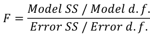](https://bookstack.mitchellhenschel.com/uploads/images/gallery/2022-08/image-1661960255081.png) The numerator df is for the model and the denominator df is for error. In a situation with one 1 X variable, the F-test is equivalent to the t-test for the null hypothesis that β1 =0. Also notice that in the case of one predictor, F is the square of t.