Survival Analysis I
Survival analysis is a measure of time until an event occurs. It doesn't only measure death as an outcome, and can adjust for covariates just as a logistic regression. But while a logistic regression only requires knowledge of whether an outcome occurred, survival analysis requires knowledge of the time until the outcome occurred.
This is usually used in a longitudinal cohort study; not common in case control studies as there is no accurate time information.
Survival Data
Survival data contains: entry time, whether the person had the event (dichotomous), and the time between when the person had the event or was last known to be event-free; as well as any other covariates (race, gender, age, etc).
Even those who drop out of the study before the outcome occurs can provide information to the study. They are assumed to have the same likelihood of death as subjects with similar characteristics who survived at least the same amount of time.
Censoring
Censoring is removing a subject before we can measure the outcome.
Type I Censoring: Observations censored after some fixed length of follow-up.
Type II Censoring: Observations censored after a fixed percentage of subjects have the event of interest.
Random Censoring: Observations censored for reasons outside the control of investigators (e.g. drop-outs).
Informative Censoring: People censored that would have had different outcomes as people who remained in the analysis for the same amount of time.
Non-informative Censoring: People censored who would have had similar risk for the outcome as people who remained in the analysis for the same amount of time. Basic survival analysis assumes that censoring is non-informative.
Right-Censored: Lower limit on the time to an event for censored subjects (more common)
Left-Censored: An upper limit on time to event (less common, also called interval-censored with both upper and lower limits)
Survival Analysis vs. Alternatives
Linear Regression
If we have a continuous dependent variable, there are several issues with using a linear regression with time to event or censoring as outcome:
- Censored observations can't be incorporated
- Distribution of survival time is usually highly skewed since some people nearly always survive a long time
- Disease status can't be handled
Logistic Regression
Neither time to event nor censoring are relevant in a logistic regression; the time between exposure and outcome is very short, and people cannot "drop out" of the study since they are recruited after the outcome is known.
Survival Function
Measures: Let T = survival time to event
Survival probability: S(t) = Pr (T > t) = Pr(the probability that an event has NOT occurred until time 't')
- S(t=0) = 1 (all survive at the start)
- S(t=inf) = 0 (non-one survives at infinity time)
- 0 <= S(t) <= 1
- S(t) is non-increasing function S(t1) >= S(t2) for t1 <= t2
Failure Function
T = survival time to event
Failure probability - the probability that event occurred by time 't'
F(t) = Pr(T <= t)
Relationship between survival function and failure function S(t) = 1 - F(t)
Hazard Rate
Instantaneous failure rate
$$ h(t) = \lim_{\Delta t \to 0 } {{Pr(t < T \le t + \Delta t | T > t)} \over {\delta t}} $$
$$ H(t) = \int h(t)*d(t) $$
Relationship between hazard and survival functions:
$$ h(t) = {f(t)} \over {S(t)} $$
f(t) = density of time to event
Cumulative hazard = H(t) = -ln(S(t))
Kaplan-Meier Curves
Kaplan-Meier curves (AKA Product-Limit Estimate) is a non-parametric approach. No assumptions on shape of the underlying distribution for survival time.
Example with censoring: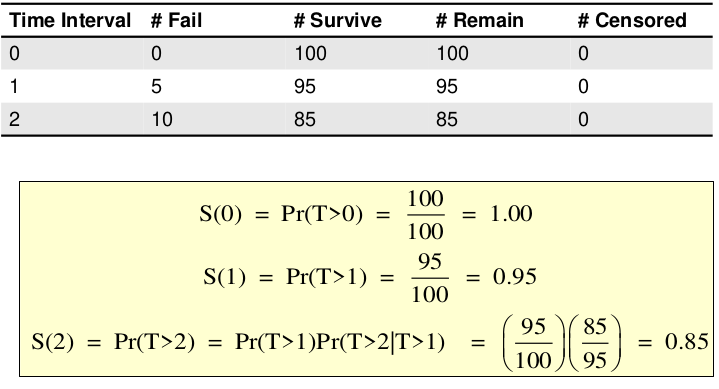
Example with censoring: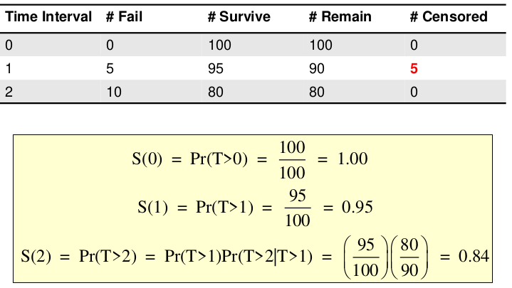
Summary Measures
- Median survival - smallest survival time for which S(t) < .5
- Sometimes this cannot be estimated
- Mean survival
- Often biased
- Hazard Ratio - cannot be estimated from the KM curve and it depends on the proportional hazards assumption
Log-Rank Test
A non-parametric crude comparison among several groups. Test whether two survival curves are statistically different by comparing observed events with expected events under the null hypothesis of no difference. Can be thought of as a time-stratified C.M.H. test.
H0: There is no difference between the populations in the probability of an event at any point in time
At the jth failure time: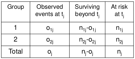
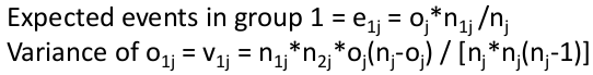
Where o = observed and e = expected
Total observed events in group 1: O1 = Sum of o1j for all j
Total expected events in group 1: E1 = Sum of e1j for all j
Variance of O1 = sum of v1j for all j
Log Rank Statistic: (O1 - E1)2 / V ~ X2 (1 df)
Proportional Hazards
An assumption of the Log-Rank test is "proportional hazards", that the hazard functions in different groups are proportional.
The survival distributions crossing is an indication of the non-proportional hazards.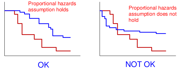
In the next chapter we will learn a formal test for proportional hazards
Regression Models for Survival Analysis
Kaplan-Meier estimator allows for crude comparison, but it does not provide an effect estimate nor does it allow adjustment for covariates.
We model the hazard as a function of the exposure and quantify the relative hazard. The hazard ratio is the effect estimate, and it allows adjustment for covariates.
T = time to event
Survival Distribution: S(t) = Pr(T > t) = Pr(Subject survives at least to time t)
Hazard function: Instantaneous failure rate, event rate over a small interval of time. Not a probability, can be greater than 1.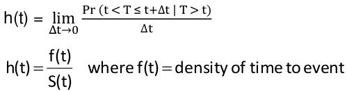
Proportional Hazards Models
The exponential model describes the hazard function as:
= basline hazard * effect of covariates
baseline hazard is a constant (it does not change with time)
R Code
### KM Curves and Log-Rank Test
fit.2 <- survfit(Surv(chdtime, chd_sw) ~ GLI, data=framdat3)
summary(fit.2)

# Kaplan-Meier Plot
plot(fit.2, mark.time=T, mark=c(1,2), col=c(1,2), lwd=2, ylim=c(0,1),
             xlab="Time (years)", ylab="Disease free survival", cex.axis=1.5, cex.lab=1.5)
legend(x=1, y=0.40, legend=c("No GLI","GLI"),
             col=c(1,2), lwd=2, cex=1.2)

# Log-Rank Test
survdiff(Surv(chdtime, chd_sw) ~ GLI, data=framdat3)

### A fancier survival plot using the **survminer** package
#### Reference https://rpkgs.datanovia.com/survminer/index.html
library(survminer)
ggsurvplot(
  fit.2,
  data = framdat3,
  xlab="Time (years)",
  size = 1,                 # change line size
  palette =
    c("#FF3333","#0066CC"),       # custom color palettes
  conf.int = TRUE,          # Add confidence interval
  pval = TRUE,              # Add p-value
  risk.table = TRUE,        # Add risk table
  risk.table.col = "strata",# Risk table color by groups
  legend.labs =
    c("GLI=0", "GLI=1"),    # Change legend labels
  risk.table.height = 0.3,  # Useful to change when you have multiple groups
  ggtheme = theme_bw()      # Change ggplot2 theme
)
No Comments