Model Fit & Concepts of Interaction

Review: Logistic and Proportional Hazards Regression Model Selection

You can look at changes in the deviance (-2 log likelihood change)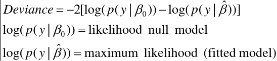

• Deviance - Residual sum of squares with normal data
  • Problem: Deviances alone do not penalize "model complexity" (hence need LRT - but only applies to nested models)
• AIC, BIC - More commonly used
  • Larger BIC and AIC -> worse model
  • BIC is more conservative
  • Both based on likelihood
  • An advantage is that you do not need hierarchical models to compare the AIC or BIC between models
  • A disadvantage is there is no test nor p-value that goes with comparison of models
  • A model with smaller values of AIC or BIC provides a better fit
  • Used to compare non-nested models
    
    • A non-nested model refers to one that is not nested in another; The set of independent variables in one model is not a subset of the independent variables in the other models
    • The data must be the same

Risk Prediction and Model Performance

How well does this model predict whether a person will have the outcome? Generally only for dichotomous outcomes, especially in genetics.

• Calibration - Quantifies how close predictions are to actual outcomes - goodness of fit
  • Models for which expected and observed event rates in subgroups are similar are well-calibrated
• Discrimination - The ability of the model to distinguish correctly between the two classes of outcome

Logistic

• A model that assigns a probability of 1 to all events and 0 to non-events would have perfect calibration and discrimination
• A model that assigns a probability of .51 to all events and .49 to all non-events would have perfect discrimination and poor calibration

Hosmer-Lemshow Test

The Hosmer-Lemshow Test is a statistical goodness of fit test for logistic regression models. It is frequently used in risk prediction models. It assesses whether or not the observed event rates match expected event rates in subgroups of the model population of size n. Specifically, it identifies subgroups as the deciles of size n_j based on fitted risk values.

H₀: The observed and expected proportions are the same across all groups

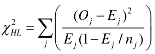
• O_j and E_j refer to the observed events and expected events respective in the j^th group
• n_j refers to the number of observations in the j^th group
• Sensitive to small event probabilities in categories
• Sensitive to large sample sizes
• Problems: Results immensely depend on the number of groups and there is no theory to guide the choice of that number. It cannot be used to compare models.

ROC: Receiver Operating Curve / C Statistic

Plots sensitivity (true positive) for different decisions and look for best trade off between sensitivity and specificity (true negative). The curve is generated using signal detection applications.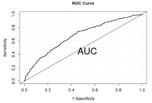

The area under the curve (AUC) is a summary measure called the c statistic, which is the probability that a randomly chosen subject with the event will have a higher predicted probability of the event than a randomly chosen subject without the event (a measure of discrimination).

• > .8   - very good
• > .75 - good
• > .7   - acceptable
• > .65 - weak
• > .6   - poor
• < .6   - useless

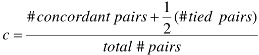
The c statistic groups all pairs of subjects with different outcomes and identifies pairs where the subject with the higher predicted value also has the higher outcome concordantly. Pairs where the subject with the higher predicted value has the lower outcome are discordant.

When we use the c-statistic in the data used to build the model it cannot be interpreted as the "true" predictive accuracy. It is simply a measure of goodness of fit.

Real predictive accuracy can be estimated when you have a new data set that is not used to generate the model. If that is not possible, inter-validation can be considered:

• Random split - Random splitting of the sample into training and validation many times (100+)
• Cross-validation - Dividing the sample into k sub-samples and train the model on k-1 samples then validate on the remaining sample and repeat many times
• Bootstrap - Resampling with replacement a new version of your sample, where each observation has the same probability of selection. The new sample is used for analysis many times

Survival Analysis

• Calibration at large - compares how close the mean of the model-based predicted probabilities at time t is to the Kaplan-Meier estimate at time t
• Calibration by decile - replace rates/proportions in deciles with their Kaplan-Meier equivalents; change degrees of freedom to 9
• c-statistic has several extensions to survival data, the most popular is Harrell's:
  • Call any two subjects comparable if we can tell which one survived longer
  • Call two subjects concordant if they are comparable and their predicted probabilities of survival agree with their observed survival times
  • 'c' defined as the probability of concordance given comparability

Interaction Analysis

Interaction is when the effect of an exposure depends on the presence or absence of another exposure, or on the level of another exposure variable.

• If there is an interaction:
  • We say there is an interaction between the two exposures
  • We cannot provide a single summary measure
  • A treatment may be beneficial to some subgroups but harmful to other subgroups
  • Sometimes helps clarify the mechanisms for outcome
• When the interaction is model dependent:
  • Evaluation of interaction depends upon the measures you are using to examine the association between exposure and disease
  • Risk differences vs ratio measures lead to different concepts of interaction

Effect Modification

There is a difference between interaction and effect modification but I will not go into detail here.

One 'exposure' is a non-modifiable background variable such as a demographic variable (a 'moderator'). The moderator affects the size and/or direction of the association between a primary exposure and an outcome.

Ex. Sex may be a moderator of the association between hypertension and heart disease, as reflected by the difference in risk ratios between men and women.

Statistical vs. Biological Interaction

• Biological interaction, or mechanistic interaction, is when two exposures are part of the same causal mechanism
• Statistical interaction is interaction in a statistical model (the focus below)
  • It is model and scale dependent: a model for risk differences may indicate an interaction while a model for risk ratios indicates no interaction, or vice versa
  • The presence of a statistical interaction does not mean there is necessarily any mechanistic or biological interaction

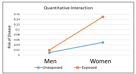
Quantitative Interaction

Quantitative interaction is when the direction of the effect of an exposure on an outcome is the same for different subgroups but the size of the effect differs.

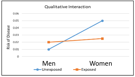
Qualitative Interaction

Qualitative interaction is when the direction of the effect of an exposure on an outcome changes for different subgroups.

Additive Interaction

Note: In the following sections we ignore sampling variability. We'll assume we have very, very large samples or an entire population.

Suppose we have two binary exposures A and B with risk: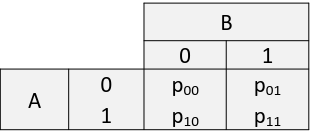

There is interaction on the additive scale if the effect of the two exposure together is not equal to the sum: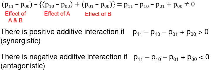

Example: Suppose we have two binary exposures A and B that have the following risk table: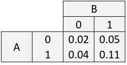

The risk difference compared to those with neither exposure: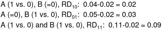

Note that RD₁₁ > RD₁₀ + RD₀₁ (Synergistic)

Risk Ratio Difference

Recall that a risk ratio of 1 means no risk.

For risk ratios: There is an interaction on the additive scale if the effect of the two exposures together is not equal to the sum of their individual effects: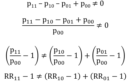

Thus, there is an interaction on the additive scale if the deviation from 1 (the null value) of the risk ratio for both exposures is not equal to the sum of deviations from 1 of the individual risk ratio for each exposure separately.

The important thing to remember here is the additive interaction can be assessed based on risk ratios without the having underlying risks.

Relative Excess Risk Due to Interaction

So there is not interaction on the additive scale if: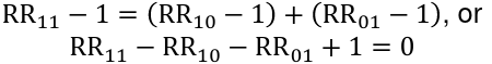

The quantity, R₁₁ - R₁₀ - RR₀₁ + 1, is called the relative excess risk due to interaction or RERI:

There is interaction on the additive scale if the RERI != 0
> 0 means positive additive interaction
< 0 means negative additive interaction

Multiplicative Scale

Suppose we have a table of risks similar to the additive risk above.

There is an interactive on the multiplicative scale if the effect of the two exposures together is not equal to the product of their individual effects:

It is possible to have both additive and multiplicative interaction, or a positive additive interaction and negative multiplicative interaction.

Case Control Studies

Additive Scale

If the outcome is rare, so that ORs estimate RRs, then we can say there is additive interaction if:

We can define the relative excess risk due to interaction as:

There is interaction on the additive scale if RERI != 0
> 0 means positive additive interaction
< 0 means negative additive interaction

Multiplicative Scale

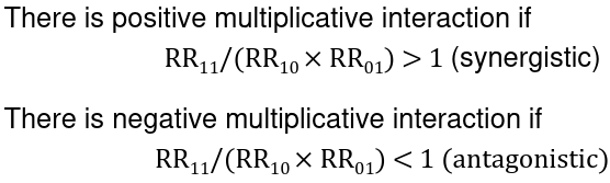
In this setting multiplicative interaction exists when:
OR_11 != OR1_10 * OR_01

OR_11 / OR1_10 * OR_01
> 1 means positive multiplicative interaction
< 1 means negative multiplicative interaction

Note this is only based on odds ratios, there is no multiplicative interaction between risk ratios, unless the outcome is rare and ORs approximate RRs.

Additive vs Multiplicative Interaction

• Direction of interaction may depend on the scale
• If both exposures affect the outcome then there is necessarily interaction on one of the scale
  • There is no interaction on either scale then one of the exposures must have no effect on the outcome
• It is argued additive interaction is the more important public health measure

Modeling with Interaction

Hierarchical models always have the lower order terms before considering higher order terms

Ex. Hierarchical: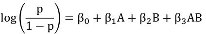

Ex. Non-Hierarchical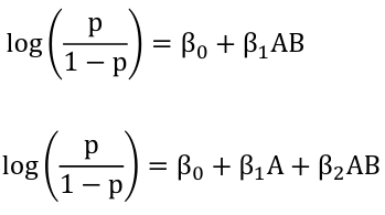

When there is no interaction term in a model the log(odds ratio) remains constant.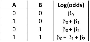

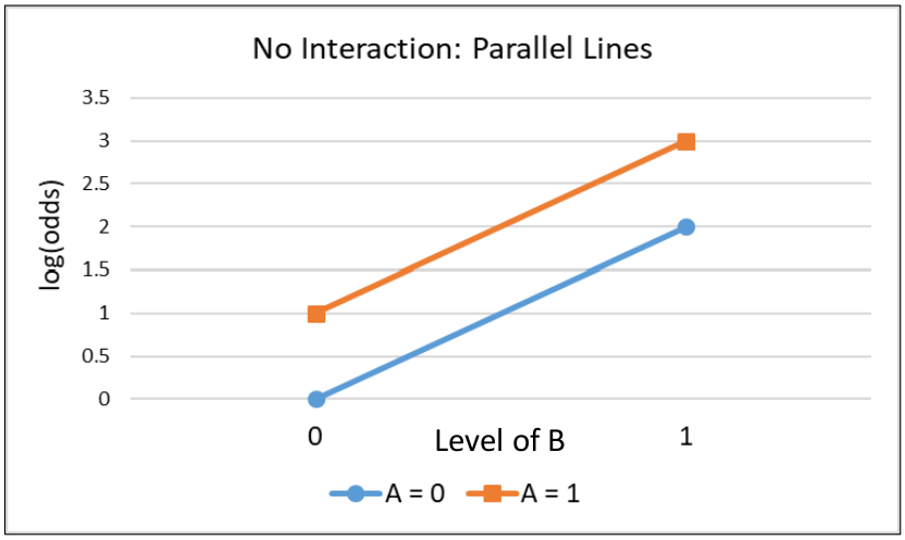
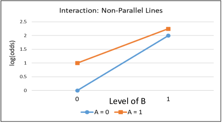
When there is an interaction term the log odds ratio is NOT constant. There is also interaction on the multiplicative scale.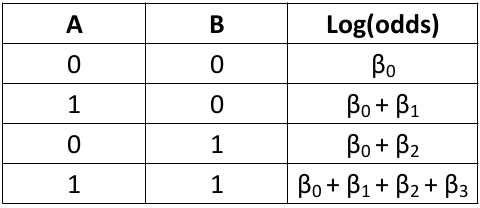

Synergy: If beta_3 > 0 the joint effect of A and B is greater than the product of the individual effects.
Antagonism: If beta_3 < 0 the joint effect of A and B is less than the product of the individual effects.

The odds ratios (the group with neither exposure as the reference):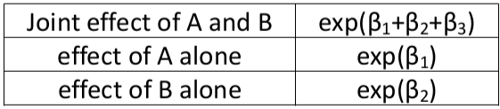

If there is an interaction term, the main effects cannot be interpreted alone, but are relative to the state of other variables.

R Code

library(effects) # To plot interactions
library(survival) # load survival package

# Hosmer-Lemshow Test
mod <- glm(y~x, family=binomial)
hl <- hoslem.test(mod$y, fitted(mod), g = 10)