Logistic Regression

Stratified analysis can be used to adjust for confounding, but the results can be difficult to adjust multiple confounders. If we have too many strata, we could end up with very small tables or 0 counts for some cells. We can instead use Logistic Regression when the following situation exists:

• The design is cross-sectional, case-control, cohort, or clinical trial
• The outcome (D) is dichotomous
• Any type of exposure (continuous, categorical or ordinal)
• Confounders/covariates can be continuous, categorical or ordinal

Goals of Logistic Regression

• Association: Between an outcome and a set of independent variables
• Prediction: What do we expect the probability of outcome to be given the set of independent variables?
• Exploratory: What variables are associated with outcome?
• Adjustment for Confounding: Focus on a particular relationship; the other variables in the model are there for adjustment

Properties of Exponential and Logarithmic Functions

• y = exp(x)   ->   log(y) = x
• exp(x)*exp(z) = exp(x + z)
• exp(x)/exp(z) = exp(x - z)
• log(a*b) = log(a) * log(b)
• log(a/b) = log(a) - log(b)

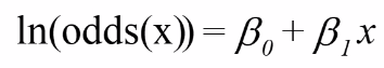
Logistic Regression Model

We assume a linear relationship between the predictor variable(s) and the Log-odds of an event that Y = 1:

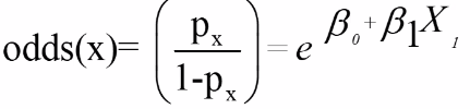
Thus, for risk p (if the design is appropriate):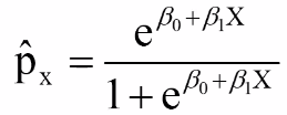

The predicted value of p is always between 0 and 1 and has a S-shaped curve. 

Properties of Logistic Model with 1 Predictor: Case-Control Study

The log odds should be a straight line as given by: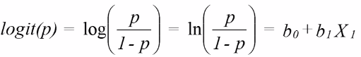

So if we have a X variable that is either 1 or 0 then the model would be:
    logit(p | x = 0) = b₀    or     log(p | x = 1) = b₀ + b₁*1

With E being exposure and bar(E) being non-exposure, we can define the odds ratio as: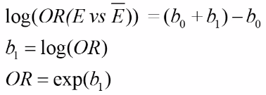
This represents the odds or log odds of developing disease with a dependent variable with one predictor in a case-control study.

In general: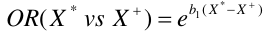

We can calculate confidence intervals for b: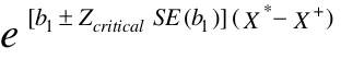

This will also hold true for more than one covariate in the model. But this is not true for the RR.

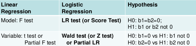
Testing the Model

Two levels of testing:

1. Test of the model
2. Test of specific variables in the model

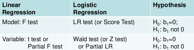
Likelihood Ratio Test

We can use the Maximum Likelihood test to estimate coefficients. Improvements in the likelihood by using the model with covariate instead of just the intercept. We use the Likelihood Ratio (LR) test when we do not know the distribution of LR.

H0: Model is x;
Ha: Model is x + all parameters

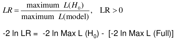
-2 ln(LR) has a chi-squared distribution with df = difference in number of parameters in the null and full models, assuming a large sample.

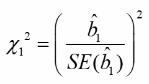
The LR, Wald, and Score test all measure the same hypothesis. For large sample sizes, they should all be equivalent. For small sample sizes LR is preferred.

LR test: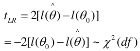

Score test: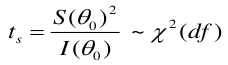

Wald test: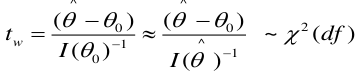

Multiple Covariates

As in multiple linear regression, the objective is to study the association by adjusting for confounding.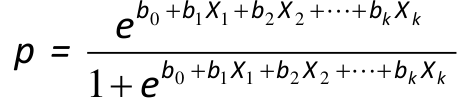

The joint effects of two independent variables is the multiplication of their individual effects (odds is the numerator from above).

We should remove missing values before analysis or apply other methods to consider missing data.

Partial Likelihood Ratio Test (PLRT) of a Specific Variable

PLRT is used to test the significance of a group of variables.

1. Run model with all variables
2. Run model with all except variable of interest
3. Compare the model chi-square statistic or likelihoods, provided the sample sizes are the same

PLRT is almost equivalent to the Wald test. Often we use multiple dummy variables to code for a continuous covariate by putting the domain into "bins".

Confounding

Our measure of association for confounding: OR_Crude / OR_Adjusted
If the ratio is > 1.1 we conclude the factor confounds the association between X and Y.

In logistic regression the 10% rule of thumb should not be applied to beta.

R Code

#### This chunk of code 
* reads data, 
* extract records with complete data
* selects records for *FEMALES* and those with *CHD=0 OR CHD>4*
```{r }
   
framdat2 <- read.table("framdat2.txt",header=T, na.strings=c("."))
names(framdat2)

work.data <- na.omit(framdat2[,-c(3,4)]) ## drop DTH and CAU columns and remove rows with missing data 
work.data <- subset(work.data, (work.data$SEX == 2) & (work.data$CHD==0 | work.data$CHD > 4))
work.data$chd_sw = work.data$CHD >= 4  ## 1 is event, 0 is no event
``` 

#### CRUDE ANALYSIS
We fit the model with only GLI, using the glm() function. "family=binomial" indicates that this is a logistic regression model.
```{r}

mod.crude <- glm(chd_sw ~ GLI, family=binomial, data=work.data)
summary(mod.crude)

```

##### Output for ORs, and Wald tests using the *aod* package
```{r }     
confint.default(mod.crude)
exp(cbind(OR = coef(mod.crude), confint.default(mod.crude))) 
library(aod) # inlcudes function wald.test()
wald.test(b = coef(mod.crude), Sigma = vcov(mod.crude), Terms = 2)
```

#### ADJUSTED ANALYSIS
model with only confounder
```{r }   
mod.age <- glm(chd_sw ~ AGE, family=binomial, data=work.data)
summary(mod.age)
```

#### model fit and summary of parameter estimates - adjusted model 
```{r }
mod.age.adjusted <- glm(chd_sw ~ GLI + AGE, family=binomial, data=work.data)
summary(mod.age.adjusted)
summary(mod.age.adjusted)$coefficients
```

##### to produce the LRT, use the anova function
```{r }
anova(mod.age, mod.age.adjusted)
```

##### estimate of adjusted OR and confidence intervals
```{r }
# regression coefficients
confint.default(mod.age.adjusted)

print( "Adjusted OR and 95% CI")
exp(cbind(OR = coef(mod.age.adjusted), confint.default(mod.age.adjusted)))  
wald.test(b = coef(mod.age.adjusted), Sigma = vcov(mod.age.adjusted), Terms = 2)
```

##### Question: is there confounding?
```{r }
exp(coef(mod.crude)["GLI"])/exp(coef(mod.age.adjusted)["GLI"])
```

#### Interpretation of fitted values
```{r }
log.odds.CHD <- log(mod.age.adjusted$fitted.values/(1-mod.age.adjusted$fitted.values))
plot(work.data$AGE,log.odds.CHD,xlab="Age", ylab="log-odds-CHD")
points(work.data$AGE[work.data$GLI==1],log.odds.CHD[work.data$GLI==1],col=2)

odds.CHD <- mod.age.adjusted$fitted.values/(1-mod.age.adjusted$fitted.values)
plot(work.data$AGE,odds.CHD,xlab="Age", ylab="odds-CHD")
points(work.data$AGE[work.data$GLI==1],odds.CHD[work.data$GLI==1],col=2)
   
```

####  model with multiple confounders -- model fit and summary of parameter estimates
```{r }
mod.adjusted <- glm(chd_sw ~ GLI + AGE + CSM + FVC + MRW + SPF, family=binomial, data=work.data)
summary(mod.adjusted)
exp(cbind(OR = coef(mod.adjusted), confint.default(mod.adjusted)))  
wald.test(b = coef(mod.adjusted), Sigma = vcov(mod.adjusted), Terms = 3)
```

##### fit model with only confounders   
```{r }
mod.confounders <- glm(chd_sw ~ AGE + CSM + FVC + MRW + SPF, family=binomial, data=work.data)
summary(mod.confounders)
anova(mod.confounders,mod.adjusted)
```