Poisson Regression

We use the Poisson Regression to model a risk ratio when we are interested not in whether something occurs but how many times it occurs; Either repeated events or events in a population.Ex. number of hospitalizations, number of infections, etc.

This assumes independent events and equal risk over time (flat hazard)

Logistic regression produces odd ratios (which approximates risk ratio when outcome is rare), but only analyzes patients with at least 1 event and can be difficult to interpret when outcome is not rare. Survival analysis can be used to analyze the time to the first event.

Poisson Distribution

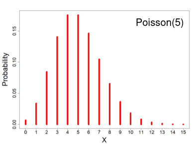
• X ~ Poisson(μ); μ  > 0
• X = the number of occurrences of an event of interest, with parameter μ
• Probability mass function
  

  

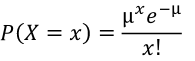
• E(X) = μ 
• V(X) = μ 

The distribution depends of the expected number of events, since the mean = variance. As the number of expected number of events increases it the more closely the Poisson distribution approximates the normal distribution.

If X ~ Binomial(n, p) and n -> inf, p -> 0 such that np is constant; X ~ Poisson(np)

Distribution of the sum of independent Poisson random variables. If Xi ~ Poisson(μi) for i = 1 to m, and the Xi's are independent then: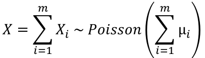

IR = (number of events)/(number of controls OR interventions)
Incident Rate Ratio = IR_intervention / IR_controls

CI for expected number of events (μ):
μ_L, μ_U = X +/- 1.96 * sqrt(X)

CI for Incidence Rate: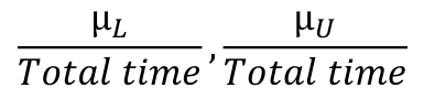

The event rate can also be written as:
    λ = μ / N
Where μ  is the expected number of events and N is the number of exposure units

We model the relationship on the log scale: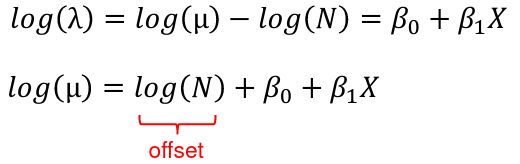

So to use the Poisson model we need 3 things:

1. Predictor variables and covariates X1, X2, X3...
2. The number of events for each "subject", defined as the group to which the event count belongs
3. The denominator that the events are drawn from Ni

For specific values of X, X*, X+:

For a CI for IRR(X* vs X+):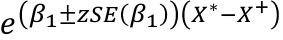

Overdispersion

Overidispersion is when the variance is greater than the mean, and is a significant problem for Poisson regression. Outliers can lead to large variances, and unmeasured effect modifications and confounders. Uncontrolled overdispersion results in model where the p-values are too small.

The solution is scaling the data to fix the standard error, the estimate is unchanged but the p-value is fixed.

Alternatives

Negative Binomial Regression

Evidence of under-dispersion (small deviance) or overdispersion (large deviance) indicates inadequate fit of the Poisson model or improper variance specification. Mean = variance requires a homogenous population, having a heterogenous population will introduce additional variance. 

NBR is used in cases where there is overdispersion in a Poisson regression:
    Variance = mean + k*mean^2 (k>=0)
The negative binomial distribution reduces to Poisson when k = 0; Where k is the number of variables.

We can test if the NBR fits the data better than the Poisson regression. One such way is a likelihood ratio test (LRT):

1. Run the first model with K variables, and record the -2Log Likelihood
2. Run the second model with K+P variables and record the -2Log Likelihood
3. Calculate the difference in the -2Log Likelihood
4. The difference is the chi-sqaure distributed with P degrees of freedom

H₀: k = 0; H_a: k>0

Zero-Inflated Poisson Models

In cases where the number of subjects with no events exceeds the expected we can consider a model where we split analysis into 2 parts:

• Look at the probability of events vs none using logistic regression
• Given at least one event, model the number of events using Poisson regression model
• The logistic and Poisson model parts are estimated at the same time
• The risk factors for having any events don't have to be the same risk factors that predict how many events happen

This will not be covered in detail here.

Risk Ratio Regression

Epidemiologists prefer risk ratios over odds ratios, as they are more intuitive. It is argued since the odds ratio estimates the risk ratio when the outcome is rare there is no good justification for fitting logistic regression models to estimate odds ratios, log binomial or Poisson are greatly preferred.

Logistic regression models the odds: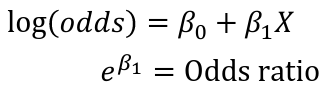

Log-binomial can be used to model the risk: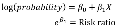

Note that the log of a probability is always negative.

• Generally log-binomial and Poisson regression models appear to have difficulties when prevalence is high (when odds ratios and risk ratios are most different).
• Poisson regression models are somewhat sensitive to outliers
• Log binomial models are very sensitive to outliers

R Code

library(epitools)
library(aod) # For Wald tests
library(MASS) # for glm.nb()
library(lmtest) # for lrtest()
library(gee) # for gee()
library(geepack) # for geeglm()

## Poisson regression
### Import data
patients <- read.csv("patients.csv", header=T)


### Poisson regression: crude model
mod.p <- glm(NumEvents ~ Intervention, family = poisson(link="log"), offset = log(fuptime), data=patients)
summary(mod.p)
confint.default(mod.p)
exp(cbind(IRR = coef(mod.p), confint.default(mod.p))) 

### Poisson regression: adjusted model
mod.p2 <- glm(NumEvents ~ Intervention + Severity, family = poisson(link="log"), offset = log(fuptime), data=patients)
summary(mod.p2)
exp(cbind(IRR = coef(mod.p2), confint.default(mod.p2))) 

### Poisson regression with summary data
Intervention <- c(0,1)
NumEvents <- c(481,463)
fuptime <- c(876,1008)

mod.s <- glm(NumEvents ~ Intervention, family = poisson(link="log"), offset = log(fuptime))
summary(mod.s)
exp(cbind(IRR = coef(mod.s), confint.default(mod.s))) 

## Overdispersed data
d <- read.csv("overdispersion.csv", header=T)

mod.o1 <- glm(n_c ~ as.factor(region) + as.factor(age), family = poisson(link="log"), offset = l_total, data=d)
summary(mod.o1)
# Joint tests:
## Test of region
wald.test(b = coef(mod.o1), Sigma = vcov(mod.o1), Terms = 2:4)
## Test of age
wald.test(b = coef(mod.o1), Sigma = vcov(mod.o1), Terms = 5:6)

# Estimate dispersion parameter using pearson residuals
dp = sum(residuals(mod.o1,type ="pearson")^2)/mod.o1$df.residual
# Adjust model for overdispersion:
summary(mod.o1, dispersion=dp)


# Estimate dispersion parameter using deviance residuals
dp2 = sum(residuals(mod.o1,type ="deviance")^2)/mod.o1$df.residual
# Adjust model for overdispersion:
summary(mod.o1, dispersion=dp2)

### Adjust for overdispersion using quasipoisson
mod.o2 <- glm(n_c ~ as.factor(region) + as.factor(age), family = quasipoisson(link="log"), offset = l_total, data=d)
summary(mod.o2)
## Test of region
wald.test(b = coef(mod.o2), Sigma = vcov(mod.o2), Terms = 2:4)
## Test of age
wald.test(b = coef(mod.o2), Sigma = vcov(mod.o2), Terms = 5:6)

### Negative Binomial regression
# Note the offset is now added as a variable
# Allow for up to 100 iterations
mod.o3 <- glm.nb(n_c ~ as.factor(region) + as.factor(age) + offset(l_total), control=glm.control(maxit=100), data=d)
summary(mod.o3)
## Test of region
wald.test(b = coef(mod.o3), Sigma = vcov(mod.o3), Terms = 2:4)
## Test of age
wald.test(b = coef(mod.o3), Sigma = vcov(mod.o3), Terms = 5:6)

### LRT to compare Poisson and Negative Binomial models
lrtest(mod.o1, mod.o3)

# Not this:
anova(mod.o1, mod.o3)

## Risk Ratio regression
ACE <- read.csv("BU Alcohol Survey Motives.csv", header=T)

oddsratio(table(ACE$OnsetLT16, ACE$AUD), rev='both', method='wald')

riskratio(table(ACE$OnsetLT16, ACE$AUD), method='wald')

### Log-Binomial model
# Crude
mod.lb1 <- glm(AUD ~ OnsetLT16, family = binomial(link="log"), data=ACE)
summary(mod.lb1)
exp(cbind(RR = coef(mod.lb1), confint.default(mod.lb1))) 

# Adjusted (did not converge)
#mod.lb2 <- glm(AUD ~ OnsetLT16 + as.factor(Sex) + as.factor(ACEcat3) + Age, family = binomial(link="log"), data=ACE)

### Modified Poisson
# Crude using gee()
mod.mp1 <- gee(AUD ~ OnsetLT16, id=id, family = poisson(link="log"), data=ACE)
summary(mod.mp1)

# Crude using geeglm()
mod.mp1.2 <- geeglm(AUD ~ OnsetLT16, id=id, family = poisson(link="log"), data=ACE)
summary(mod.mp1.2)

# Adjusted using gee()
mod.mp2 <- gee(AUD ~ OnsetLT16 + as.factor(Sex) + as.factor(ACEcat3) + Age, id=id, family = poisson(link="log"), data=ACE)
summary(mod.mp2)

# Adjusted using geeglm()
mod.mp2.2 <- geeglm(AUD ~ OnsetLT16 + as.factor(Sex) + as.factor(ACEcat3) + Age, id=id, family = poisson(link="log"), data=ACE)
summary(mod.mp2.2)