Survival - Time to Failure
Analysis of survival data is more complex than than other methods we've seen so far; We can't just take the mean survival time a a confidence interval to predict when the last patient will die. Also, survival times are unlikely to follow a Normal distribution, so simple regression techniques are not applicable.
Censoring
Censoring of data can happen in a number of ways:
- Some subjects still have not experienced the event of interest by the end of the study. Most studies have a recruitment period followed by a pure follow-up period. Patients who are enrolled earlier have a higher chance of experiencing the event.
- Some participants drop out early, either due to dropping out or another event unrelated to the study.
In either case, you know that the subject has participated in a study to a certain time without witnessing the event, but have no information thereafter. Such incomplete information is said to be right censored. Note that we censor the data, not the subject. Throughout this lecture we will assume independent censoring - the participants remaining in the study are representative of the target population.
Methods of Analyzing Survival
Let's consider a dataset of rats testing a new cancer treatment.
Approach 1: Test for Difference in Outcome After a Set Time (Wrong)
We could pick a set number of days and consider the number of rats in each group. We can use a chi-square test to determine if the outcome between the two groups is the same. A 95% confidence interval for the population could also be determined.
The problem with this approach is it disregards exact death times and ignored censored observations before the cutpoint. Comparing survival at a single point in time is not informative, the results could change significantly at a different cutpoint.
Approach 2: Comparing Incidence Rates
Estimates can be obtained for the incidence rates, by taking the number of deaths and the population follow-up time in each group. We would expect the proportion of cases will be the same under the null hypothesis. The estimate of the rates can also be obtained by using a Poisson regression.
SAS Script
data one ;
input Group C Time ;
LogT = log ( Time ) ;
cards ;
1 17 4095
2 19 5023
run ;

proc genmod data = one ;
class Group ;
model C = Group / dist = poisson offset = LogT ;
estimate ’ Group 1 ’ Intercept 1 Group 1 0/ exp ;
estimate ’ Group 2 ’ Intercept 1 Group 0 1/ exp ;
Estimate ’ Group 2 vs 1 ’ Group -1 1/ exp ;
Run ;
Approach 3: Consider Follow-Up Time to be a Stratifying Variable
Compare rates between groups in the first 200 days, days 201-250 and 251-300. Dropouts/censoring occur at the end of each interval.
We could make a 2x2 table for each strata and use the Cochran - Mantel - Haenszel test statistic for Group 1 vs Group 2 survival.
/* Comparing survival using CMH test and 3 time strata */
data RCMH ;
do group =1 to 2;
Do time =1 to 3;
input yes no @@ ;
output ;
end ;
end ;
cards ;
6 13 9 4 1 1
4 17 9 8 5 2
run ;

proc sort data = RCMH ;
by group time ;
run ;

proc transpose data = RCMH out = RCMH2 prefix = count name = died ;
by group time ;
run ;

/* Comparing survival using CMH test and 3 time strata */
title1 ’ Comparing survival using CMH test and 3 time strata ’;
options pageno =1 ps =57 ls =91 center nodate ;
proc freq data = RCMH2 order = data ;
table time * group * died / cmh chisq relrisk ;
weight count1 ;
run ;
Approach 4: Log-Rank Test (Best)
Taking smaller intervals gives a more refined test. If the intervals are chosen based on the event times, that is each interval starts and ends with an event, the resulting test is the log-rank test.
Here the censored obesrvations are followed through the last interval they complete. In the data, to fully specify the each subject we must provide (1) a time of follow-up and (2) an indicator of whether censorship or the terminating event occurs at that time.
This can be performed by hand; however, it can get computationally intensive. The Log-Rank test can be directly obtained from SAS from PROC LIFETEST; the risk variable should be specified in the STRATA statement.
SAS Script
data ratc ;
input group day censor @@ ;
logt = log ( day ) ;
cards ;
1 143 0 1 220 0 2 156 0 2 239 0
1 164 0 1 227 0 2 163 0 2 240 0
1 188 0 1 230 0 2 198 0 2 261 0
1 188 0 1 234 0 2 205 0 2 280 0
1 190 0 1 246 0 2 232 0 2 280 0
1 192 0 1 265 0 2 232 0 2 296 0
1 206 0 1 304 0 2 233 0 2 296 0
1 209 0 1 216 1 2 233 0 2 323 0
1 213 0 1 244 1 2 233 0 2 204 1
1 216 0 2 142 0 2 233 0 2 344 1
run ;

title1 ’ Using Log - Rank test ’;
options pageno =1 ps =57 ls =91 centerPROC LIFETEST data = ratc notable ;
TIME day * censor (1) ;
STRATA group ;
run ;
Note that the censoring variable contains the label associated with observation being censored in parentheses.
Survival Function
Denote T as the time to event for an individual. The survival function (denoted by S(t)) is defined as:
$$ S(t) = P(T > t), 0 \leq t < \infty $$
In other words, S(t) is the probability the individual survives beyond time t.
The Cumulative Distribution Function (CDF) of the random variable T is defined as F(t) = P(T <= t) and is related to the survival function through: F(t) = 1 - S(t)
Suppose T is a continuous random variable. In this case, the hazard function λ(t), is defined as the instantaneous rate of failure at T = t conditional on surviving beyond T = t. Note the hazard is NOT a probability.
More precisely, since the probability of an event in the interval (t, t + δ) given the event has not occurred up to time t, is P(t < T <= t + δ|T > t), the hazard is obtained by dividing the probability by the length of the interval and defining a limit. In other words:
$$ \lambda(t) = \lim_{\delta \to 0+} {{P(t < T \leq t + \delta | T > t)} \over {\delta}} $$
Some simplification reduces this to F'(t) / S(t) or f(t) / S(t), where F'(t) or f(t) is the probability density function (the derivative of F(t)). From linking the survival function to the cumulative distribution function we know F'(t) = -S'(t), so we can further reduce the hazard to:
$$ \lambda(t) = d log S(t) / dt $$
and integrating both sides with respect to t and using the fact that S(0) = 1:
$$ S(t) = exp( - \int_0^t \lambda(s) ds) $$
Which gives us the cumulative hazard function:
$$ A(t) = \int_0^t \lambda (s) ds $$
Which we can simplify again to get the density function as a product of the hazard function:
$$ f(t) = \lambda(t) exp(-\int_0^t \lambda(s) ds) $$
All three parameters (survival, cumulative hazard and density) are related. If one parameter is specified the other 2 can be derived.
Life Table Estimates
Life tables are used to describe pattern of survival in populations. These methods can be applied to the study of any time to event endpoint.
The life table method requires a pre-specification of a set of intervals that span the follow-up time. The life-tables are computed by counting the numbers of censored and uncensored observations that fall into each of the time intervals.
The conditional probability of an event in the interval Ii = [ti,ti+1) given that the event did not occur up to time ti that is P(T ∈ Ii | T > ti) is estimated by:
$$ p_i = r_i / m_i $$
where r is the number of events in the interval, I and m = n - c/2 are called the effective sample size, equal to the number of patients at risk (n) in the interval m minus half the number of censored observations (c) in the interval I. This is because the assumption of the life-table is that any censored observation with an interval is treated as if it were censored at the midpoint of the interval. So, since the censored observations are at risk for only half the interval they count for only half in figuring out the number at risk.
The estimated variance of pi and its estimated standard error is:
$$ var(p_i) = {{ p_i (1 - p_i) } \over m_i} $$
The product limit estimate of the survival function at ti is obtained by piecing together the conditional probabilities pi estimated above.
$$ \hat S (t_0) = 1 $$
$$ \hat S (t_i) = P(T > t_i) = P(T < t_i | T > t_{i-1})P(T > t_{i-1}) = (1 - p_{i - 1})\hat S(t_{i-1}) =(1 - p_{i - 1})(1 - p_{i - 2})... (1 - p_{1})(1 - p_{0}) $$
$$ Var(\hat S(t_0)) = 0 $$ $$ Var(\hat S(t_i)) = \hat S(t_i)^2 \sum_{j=1}^{i-1} {p_j \over {m_j (1-p_j}}$$
The Life-Table function estimates are piecewise constant functions with estimates at the midpoint at each interval. Calculated as:
$$ h(t_{im}) = {r_i \over {w_i(n_i - {c_i \over 2} - {r_i \over 2})}} $$
Where for the ith interval, t is the midpoint, r is the number of events, w is the width of the interval and n is the number still at risk at the beginning of the interval, and c is the number of censored observations within the interval. The estimate assumes the events occur at the middle of the interval.
title ’ Angina Pectoris in Framingham study ’;
data anginaf ;
input censor time sex freq @@ ;
years =1.5+3* time ;
cards ;
0 0 1 33 0 0 2 35
0 1 1 64 0 1 2 50
0 2 1 59 0 2 2 63
0 3 1 76 0 3 2 85
0 4 1 83 0 4 2 85
0 5 1 99 0 5 2 91
0 6 1 110 0 6 2 91
0 7 1 105 0 7 2 87
0 8 1 932 0 8 2 1561
1 0 1 139 1 0 2 82
1 1 1 34 1 1 2 31
1 2 1 36 1 2 2 35
1 3 1 30 1 3 2 42
1 4 1 37 1 4 2 39
1 5 1 39 1 5 2 37
1 6 1 31 1 6 2 34
1 7 1 37 1 7 2 42
1 8 1 0 1 8 2 0
run ;

title ’ Angina Pectoris in Framingham study ’;
proc lifetest data = anginaf method = lt intervals=(1.5 to 25.5 by 3);
time Years * Censor (0) ;
freq Freq ;
strata sex ;
run ;
Kaplan-Meier Estimate
The Kaplan-Meier estimate of the life table estimate is a non-parametric estimate of S(t) with intervals being create by failure times.
Suppose we have order failure time 0 < t1 , t2 ... < tm, so that for any tk < t < tk+1. The Kaplan-Meier estimate is obtained by estimating each term separately and then multiplying the estimates. Corresponding to each tk let nk be the number "at risk" just prior to time tk and dk be the number of deaths at time tk.
An estimate of P(tk < t < tk+1 | T > tk-1) is the proportion of events in the interval (dk) among the subjects still at risk at the beginning of the interval which is nk. Thus the estimate of the proportion of deaths is \( d_k \over n_k \)
Multiply all the estimates together to get the Kaplan-Meier estimator (or the product-limit estimator) of S(t):
$$ \hat S(t) = \prod_{j | t_j < t} {{n_j - d_j}\over n_j} $$
The survival functions in each group are estimated using the Kaplan-Meier method. Often the Log transformed or Log(-Log()) transformed survival functions. If the curves are parallel between groups then proportional hazards can be employed (discussed more later).
The Wilcoxon test is another method for comparing survival curves. It is similar to Log-Rank but places more weight on early survival times while Log-Rank places more weight on later survival times.
Accelerated Failure Time Models
Let's assume a time to event outcome with 3 predictors. We want to study the association between these predictors and the distribution of a time to event outcome. In Accelerated Failure Time Models (AFTM) the response is chosen to be the Log of time to event, then we model it as a linear combination of the predictors and an error term which is scaled by a parameter sigma with a known distribution:
This resembles the classical linear regression model but we want to be able to accommodate censored data.
1. First assume the scale sigma = 1 and beta_0 = 0. Then:
Where Ti0 is a baseline time to event for X1 = X3 = X3 = 0 whose distribution is assumed known. Thus the survival times distributions for individuals with covariate values Xi1 = xi1, Xi2 = xi2, and Xi3 = xi3, is changed by a scale factor from a baseline distribution of T0.
Using this model, the survival distribution is: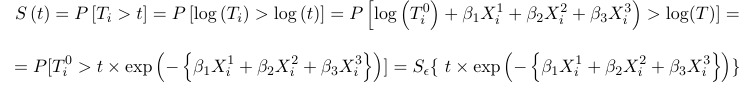
2. If we allow for a nonzero intercept and a scale parameter, then the above becomes: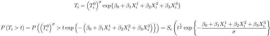
where S is the survival function of the survival time T0
Constructing the Likelihood (Assuming Right Censoring)
The time to event observations t1, t2 ... tn are assumed independent, and this the likelihood is a product of the contribution from each observation. There are two types of observations (a) censored observations and (b) event times.
a) If the observation is a censored time the the contribution is P(T > ti) = S(ti)
b) If the observation is an event time, the the contribution is f(ti) where f is the density
Thus the likelihood: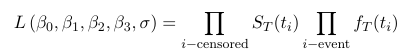
which is then maximized over theta to obtain point estimates for the betas and sigma. This is too hard to do by hand so SAS has PROC LIFEREG to fit this type of model. It assumes right censoring but other types of censoring can be accommodated.
No Comments