Gamma Regression
Consider a continuous dependent variable that is positive-valued, such as a length of a hospital stay, time waiting or the cost of a bill. This type of data is continuous in nature and oftentimes skewed and a normal approximation does not hold.
The type of data above presents a constant Coefficient of Variation (CV), that is:
$$ \sqrt{var(Y_i)} \over E(Y_i) = \sigma $$
The identity induces a quadratic variance function:
$$ var(Y_i) = \sigma^2E(Y_i)^2 $$
To model such data a number of approaches proposed in the literature have proved useful, including Log-Normal models and Gamma Regression models
- Log Normal models - the log transformation followed by a classical linear model is fairly successful in modeling this type of data. This approximation works best when the scale parameter (sigma) is small. Indeed, the log transformed model has approximately constant variance:
$$ log(Y) \approx log(\mu) + (Y - \mu) {{\delta log(y)} \over {\delta y}}(\mu) = log(\mu) + {{Y - \mu} \over \mu} $$
$$ Var(log(Y)) \approx {Var(Y) \over \mu^2 } = {{\sigma^2\mu^2} \over \mu^2 }= \sigma^2 $$ - Gamma Regression - the Gamma regression keeps the outcome on the original scale. If one wants to work on the original scale the framework of the generalized linear model proves very fruitful.
Gamma Distributions
The Gamma family is a very flexible family of distributions with support on the positive axis. The family is indexed by two parameters. One way to parameterize which is used in SAS and focused on in this lecture is called the mean parameterization.
A variable is said to follow the Gamma distribution if the density has the form:
$$ f_Y(y) = {1 \over {\Gamma (v)y} }({{yv \over \mu}})^v exp(-{{yv} \over \mu}), 0 < y < \infty $$
where
$$ \Gamma(v) = \int_0^\infty x^{v-1}exp(-x)dx $$
The mean and variance of a Gamma distributed variable are:
$$ E(Y) = \mu $$
$$ var(Y) = {\mu^2 \over v } = \sigma^2\mu^2, \sigma^2 = {1 \over v} $$
The parameter v is called the scale parameter, and \( v / \mu \) is called the rate parameter. The inverse of the scale parameter (\(\sigma^2\)) is called the dispersion parameter.
Properties of the Gamma Distribution
- The shape of the density is controlled by v
- Regardless of the value of v the densities are skewed to the right
- When v < 1 the Gamma distribution is exponentially shaped and asymptotic to both vertical and horizontal axes
- A Gamma distribution with scale parameter v = 1 and mean parameter μ is the same as an exponential distribution with mean parameter μ. In SAS we can actually test whether v = 1
- When v > 1 the Gamma distribution assumes a unimodal but skewed shape. The skewedness reduces as the value of v increases. As v tends to ∞ the Gamma distribution begins to resemble a normal distribution.
- The chi-sqaure distribution is a special case of the Gamma. A chi-sqaure distribution with n degrees of freedom is the same as a Gamma with \( v = {n \over 2} \) and \( \mu = n \)
- The Gamma is a flexible life distribution model that may offer a good fit to some sets of failure data. However, it is not widely used as a life distribution model for common failure mechanisms.
- The Gamma does arise naturally as the time-to-first failure distribution for a parellel system with components having lifetimes distributed exponentially. If there are components in the system and all components have exponential lifetimes with mean \(\gamma\), then the total lifetime has Gamma distribution v = n and \(\mu = n\gamma \)
- The Gamma distribution is widely used in engineering, science and business.
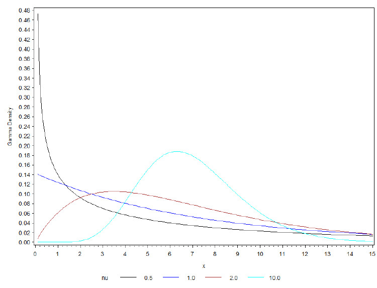
The above is an example of different shapes of the Gamma distribution with different values of v and μ = 7
Gamma as a Generalized Linear Model
As with all Generalized Linear Models, to specify the Gamma regression as a GLM we need to specify the link and variance function besides the distribution of the response.
- Variance function is V(μ) = a*μ2
- The most commonly used link function are the Log (g(μ) = log(μ)) and inverse (g(μ) = 1 / μ). The default in SAS is inverse
- With inverse link, a change in the coefficients will induce an opposite change in the expected value of the response, with log link the opposite is true
- The inverse link does not map the expected value μ into the whole real line; therefore we have to be careful when we interpret parameters
Interpretation
Assume we have a dichotomous exposure X (1 = yes, 0 = no). If the log link is used we can describe the regression as:
$$ log(\mu(X)) = \alpha + \beta*X $$
The coefficient β is interpreted in terms of Mean Ratio (MR)
$$ MR = {{exp(\alpha + \beta)} \over {exp(\alpha)}} $$
The increase in logarithm of means for one unit increase in X.
With an inverse link a change in the coefficients will induce an opposite change in the expected value of the response.
$$ {1 \over {\mu(X)}} = \alpha + \beta*X $$
The coefficient β is interpreted in terms of Inverse Mean Difference (IMD)
$$ IMD = {{1 \over \mu_{X=1}} - {1 \over \mu_{X=0}}} = \alpha + \beta - \alpha = \beta $$
One unit increase in X causes and increase of β in the inverse of means.
With log link the interpretation of the parameters is similar to the logit models; however the odds are replaced by the means, and the OR is replaced with mean ratios:
$$ log( {\mu_i \over \mu_{i'}}) = \beta(X^1_i - X^1_{i'})$$
The expected response is multiplied by exp(β) for each unit change in X1
With inverse power metric a change in the coefficients will induce an opposite change:
$$ {1 \over \mu_{i}} - {1 \over \mu_{i'}} = \beta(X^1_i - X^1_{i'})$$
The inverse of the expected response changes by β for each unit change in X. If β > 0 then the mean decreases with an increase in X, while if β < 0 then hte mean increases with an increase in X.
Measuring Goodness of Fit
The log-likelihood for a given model M: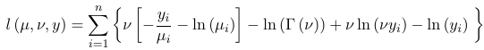
The log-likelihood for a saturated model: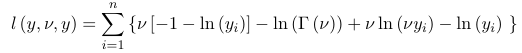
Thus the deviance is:
In Gamma regression the scaled deviance and the scaled Pearson chi-square are measures of goodness of fit statistics. For the Gamma distribution \(\sigma^2 = {1 \over v} \). If v is a known priori for a model M that has p parameters and n observations, the scaled deviance and scaled Pearson chi-square are:
$$ {D \over \sigma^2 } $$ and $$ {{X^2 \over \sigma^2} \approx \chi^2_{n-p'}}$$
That is reject the model if:
$$ {D \over \sigma^2 } > \chi^2_{n-p, 1-\alpha} $$
Where σ is estimated from the data. Thus to compare two nested models, with p and 1 parameters:
$$ {{D_{M_2} - D_{M_1}} \over \sigma^2} \approx \chi^2_{p-1} $$
These estimates can be very unstable; however, one reasonable approach is to estimate it in the largest model we are willing to consider then use that estimate in model selection.
Estimating the Dispersion Parameter
For a Gamma distributed variable Z, with Mean = E(Z) = μ and Variance = Var(Z) = 𝜎2μ2, with a response Yi for subject i we can estimate variance as:
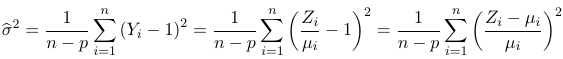
For a normal linear regression a similar result holds. The scale parameter in PROC GENMOD is the standard deviation.
Exploratory Data Analysis
To check the assumptions of a Gamma regression and to help choose an appropriate function form and link function you can plot the predictors X vs log(E(Y)) and 1/E(Y). The more appropriate link would appear linear.
With ordinal predictors you would compute the raw means of the response at each level of the predictor while for continuous outcomes you can aggregate values of predictors and treatment as ordinal.
SAS Code
/*****************************************************************/
/*** Gamma Model - Log normal                           ***/
/*****************************************************************/
title1 'Gamma regression - Saturated model';
title3 'Inverse Link';
proc genmod data=claims;
class policyholderage cargroup ageofcar ;
model lcost=policyholderage|cargroup|ageofcar @2	/dist=normal ;
weight number;
run;

/*****************************************************************/
/*** Gamma Model - Log Link                            ***/
/*****************************************************************/
title1 ' Gamma regression - Saturated model';
title3 'Log Link';
proc genmod data=claims;
class policyholderage cargroup ageofcar ;
model cost=policyholderage|cargroup|ageofcar 	/dist=gamma link=log ;
weight number;
run;
No Comments