Introduction

Generalized linear models are extensions of classical linear models. Classes of generalized linear models include linear regression, logistic regression for binary and binomial data, nominal and ordinal multi-nomial logistic regression, Poisson regression for count data and Gamma regression for data with constant coefficient of variation.

Generalized Estimating Equations (GEE) provide an efficient method to analyze repeated measures where the normality assumption does not hold.

Review

Linear Models

Classical linear models are great, but are not appropriate for modeling counts or proportions.

In SAS there are > 10 procedures that will fit a linear regression, example:

title " Simple linear regression of Income " ;
proc reg data = IM ;
model Inc = EN Lit US5 ;
output out = OutIm ( keep = Nation LInc Inc En Lit US5 r lev cd dffit )
rstudent = r h = lev cookd = cd dffits = dffit ;
run ;
quit ;

A model generally fits well if the residuals, or difference between predicted and observed, are small. The assumption of a linear model are primarily checked through the residuals (normality, homoscedasiticity/constant variance and linearity)

Normality assumption of the outcome is almost always not met in real data. One of the solutions proposed is to transform the data. The most popular methods is logarithmic.

Recall that:
    Mean(g(Y)) !=  g*Mean(Y)

GoF and Outliers

R-Squared is a measure of goodness-of-fit where higher values are indicative of a better fit.
     R² = Explained Variation  /  Total Variation
The issue with R-Squared is that more predictors will increase R² regardless of the quality of the predictor. R-Squared-Adjusted penalizes for complexity.

We do not want observations that lie on the '1%' ends of the distributions to influence the model. The leverage of an observation is defined in terms of its covariate values.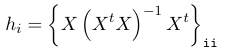

An observation with high leverage may or may not be influential;  Where we have p predictors and n observations we define leverage points as h_i > 4/n
A point with high leverage might not have high influence, that is the model does not change substantially when the point is excluded. Cook's distance can be used to identify influential points: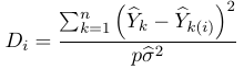
OR
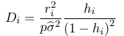
Other measures of the influence are:
DFFITTS, how much an observation has effected the fitted value: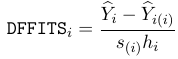

DFBETAS, the difference in each parameter estimate:  Values larger than 2/sqrt(n) should be investigated.

Model Selection

Types of models:

• Complete/Full - Reproduces data without simplification; As many parameters as observations
• Null/Intercept - Only the intercept, one predicted value for all observations
• Maximal - largest model that we are prepared to concider
• Minimal - contains minimal model parameters that must be present

1. Log-Likelihood ratio statistics
   • LR_i = 2[log L (Saturated Model) - log L_i
2. Alike information criterion
   • AIC_m = -2 ln L_m + 2k_m
3. Bayesian Information Criterion
   
   • BIC_m = -2 ln L_m + k_m * ln n

Generalized Linear Models

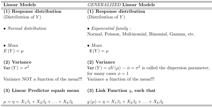
With the Generalized Linear Models, the classic linear model is generalized in the following ways:

1. Drops the normality assumption
2. Allows the variance of the response to vary with the mean of the response through a variance function
3. The mean of a population is allowed to depend on the linear combination of the predictors through a link function g, which could be nonlinear. Shown as:
   η = g(μ_i) = β₀ + β₁ X_i + β₂X_i²+ β₃ X_i³
   and η is called the linear predictor
   

With Generalized Linear Models, the classical Linear Model is generalized in a number of ways and is, therefor, applicable to a wider range of problems.