Models for Two-Way Contingency Tables
Recall in the last section Generalized Linear Models (GLMs) were introduced as an extension of the traditional linear model, it eases the assumptions in the following ways:
- Drops the normality assumption
- The response variable is allowed to follow any distribution of the exponential family (binomial, Poisson, negative minomial, gamma, multi-nomial, etc
- Assumes the variance of the response depends on a function of the mean, called a variance function
- The mean of the population is allowed to depend on the linear combination of the predictors through a link function, g
- The following link functions are used most often
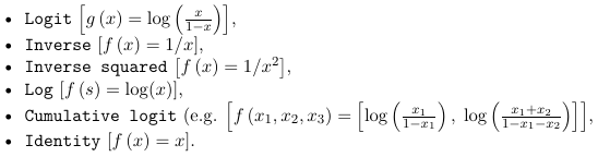
- The below table specifies which function to use with each distribution
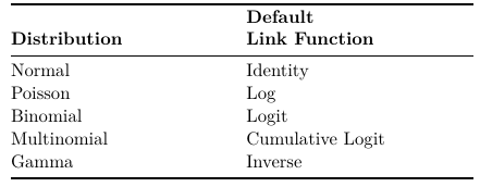
- The following link functions are used most often


In SAS
- PROC GENMOD
- The GENMOD is a procedure for analyzing generalized linear modes
- PROC LOGISTIC
- The LOGISTIC procedure is constructed for logistic regression and provides useful information
as diagnostic plots, odds ratios and other measures specific to logistic regression models.
- The LOGISTIC procedure is constructed for logistic regression and provides useful information
- PROC CATMOD
- The CATMOD procedure is a procedure designed to fit models to functions of categorical response variables.
All of these procedures report the deviance. PROC LOGISTIC reports AIC and BIC, and it can be calculated with information from PROC CATMOD.
Estimation in Generalized Linear Models
GLMs are estimated with the Maximum Likelihood (ML) method. This chooses the value which makes the observed data the most probable (equivalent to the least squares method).
Example: Let τ be the prevalence of a disease in some population. Suppose that a random sample of size 100 is selected and we observe Y = 40 individuals with the disease.
Use the data(Y) to obtain an estimate of τ_hat(Y), assuming τ has good statistical properties. By "good" it means the estimate has little to no bias and small variance.
In this example, if τ = .5 then we would write the likelihood function as:
Pτ (Y = 40) = 100C40 .540 (1 - .5)100 - 40
As a function of τ, the function Pτ(Y = ?) is called the likelihood function
Log-linear Models/Contingency Tables
Log linear models for contingency tables specify how the cell counts depend on the levels of categorical variables defining that table. Loglinear models treat all variables as symmetrically and attempt to model all important associations among them. In this sense, it's very similar to correlation analysis of continuous variables where the goal is to determine the patterns of dependence and independence among a set of variables.
Loglinear models are generalized linear models with Poisson response distribution, Log link function, and Identify variance function (for Poisson: Expected value = variance)
Data are represented in contingency tables as cell counts. The counts in the cells are assumed to follow a Poisson distribution. Loglinear models are used to model association patterns among categorical variables.
Log linear models are analogous to correlation analysis for normally distributed data, and are most appropriate when there is no clear distinction between response and explanatory variables.
Example of Contingency tables: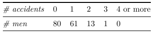
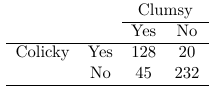
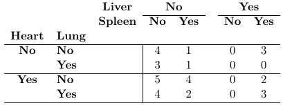
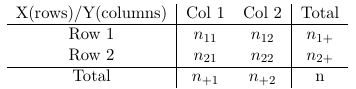
Data can be through of arising by sampling from a population and classify each individual in one of the cell of the two-way cross-classification of the two binary responses it falls in. Each count is assumed to follow a Poisson distribution with expected frequencies: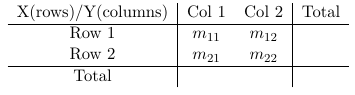
If we fix n (condition on n) the counts in the four cells follow a multinomial distribution.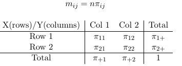
Loglinear models are constricted using the expected values (mij) rather than piij. The main distributional assumption is that nij follow a Poisson distribution with expectancy mij.
There are several different kind of loglinear models we can fit to the data above.
Saturated Model
A model that is as complicated as the number of observations. Such a model is over-specified ('less-than-full-rank-coding' or 'GLM coding'). The result does not reduce the complexity of the data and will give a 'perfect prediction'.
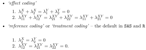
The {λX i } are called row effects, {λYj} are called column effects and { λij XY } are called interaction effects.
To solve a saturated model, the practice is to impose linear constraints on the parameters to reduce the number of parameters.
Testing Goodness of Fit in Loglinear Models
As with any other model, the GoF can be evaluated by comparing the observed to the predicted values - or the current model to the saturated model. It is not always appropriate to simply subtract the observed and fitted values!
For a loglinear model, two goodness of fit statistics are commonly used:
- Deviance Statistic

- Pearson chi-sqaured statistic
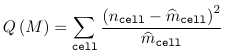
Where ncell is the observed count for a cell and m_hatcell is the fitted cell frequency in model M. Under the assumption that model M is the right model, both G2(M) and Q(M) ~ chi2(n - p), with p being the number of parameters in the model M.


Properties of the Goodness of Fit Statistic
- When the model M holds, both statistics follow a chi-squared with the degrees of freedom equal to the number of cells minus the number of estimated parameters
- The deviance (likelihood ratio) statistic can be used to test the difference between two nested models, M1 and M2
Model M1 is said to be nested in M2 (M1 ⊂ M2) if the parameters are a subset of the parameters in M2.
- The statistic G2(M1 | M2) = G2(M1) - G2(M2) will follow a chi-squared with p2 - p1 DF where p1 and p2 are the number of linearly independent parameters in models M1 and M2, respectively
Saturated Loglinear Model for SxR Table

As above, the {λi^X } are called row effects, {λj^Y} are called column effects and λij^ XY are called interaction effects.
The number of parameters in the above model will be 1 + S + R +RS. The number of observations is S*R, hence the model is over-specified. To reduce the number of parameters linear constraints are imposed on the parameters. For example, reference coding would be represented as:
λSX = λRY = 0, or
λSjXY = λiRXY for every i and j, or:![]()
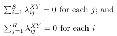
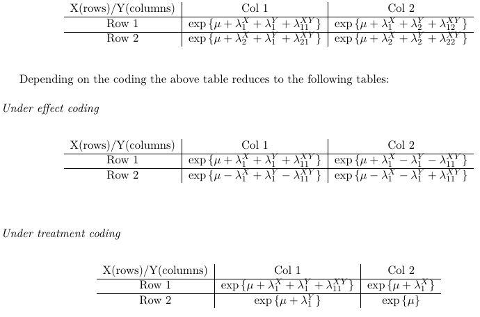
With either of these two coding constraints, the effective number of parameters for the saturated model is:
1 + (S - 1) + (R - 1) + (R - 1)(S - 1) = SR
For any number of dimensions the number of parameters in the saturated log-linear model equals the number of cells in the table. The saturated model give "perfect prediction" since it has the same number of observations as parameters.
No Comments