Hypothesis Testing with GLM
Effect modification can be modeled with logistic regression by including interaction terms. A significant interaction term implies a departure from heterogeneity between groups.
Consider the following example were we wish to compare admission rates by sex per department: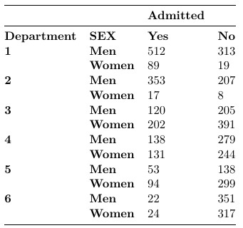
With summary of fit: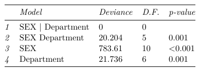
Which we observe only the saturated model fits the data well. To compare ORs across department we estimate the department specific odds from the saturated model:
ods select estimates ;
title1 ’ Estimated ODDS Ratio ( F vs M ) in each Department ’;
proc genmod data = one ;
class department SEX ;
model yes / total = SEX | department / link = logit dist = bin covb ;
estimate ’ SEX1 ’ SEX 1 -1 department * SEX 1 -1 0 0 0 0 0 0 0 0 0 0/exp;
estimate ’ SEX2 ’ SEX 1 -1 department * SEX 0 0 1 -1 0 0 0 0 0 0 0 0/exp;
estimate ’ SEX3 ’ SEX 1 -1 department * SEX 0 0 0 0 1 -1 0 0 0 0 0 0/exp;
estimate ’ SEX4 ’ SEX 1 -1 department * SEX 0 0 0 0 0 0 1 -1 0 0 0 0/exp;
estimate ’ SEX5 ’ SEX 1 -1 department * SEX 0 0 0 0 0 0 0 0 1 -1 0 0/exp;
estimate ’ SEX6 ’ SEX 1 -1 department * SEX 0 0 0 0 0 0 0 0 0 0 1 -1/exp;
run ;
The hypothesis tests we've encountered so far can be expressed in terms of linear combinations of the model parameters; However, other tests have to be carried out that may not be included in default output which requires a good understanding of the model.
For example, a few important properties we've seen so far:
- Differences between groups (Lecture 4)
Expressed as a linear combination:
1 × β1 + 0 × β2 + (−1) × β3 + 0 × β4 = 0 - Independence in 2 way tables defines by categorical variables X and Y
H0: X and Y are independent <-> H0: all λXYij = 0
HA: X and Y are dependent <-> HA: at least one λXYij != 0
Expressed as a linear combination:
λ11 = λ12 = λ21 = λ22 = 0
1 × λ11 + 0 × λ12 + 0 × λ21 + 0 × λ22 = 0
0 × λ11 + 1 × λ12 + 0 × λ21 + 0 × λ22 = 0
0 × λ11 + 0 × λ12 + 1 × λ21 + 0 × λ22 = 0
0 × λ11 + 0 × λ12 + 0 × λ21 + 1 × λ22 = 0 - Significance of parameters (Lecture 4)
Expressed as a linear combination:
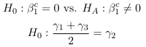
(For ordinal SBP): 0 × β0c + 1 × β1c + 0 × β2c = 0
(For SBP): γ1 + (−2) × γ2 + γ3 + 0 × γ4 = 0

In all cases the null hypothesis can be expressed as a linear combination of the parameters (this is important in understanding contrast and estimate statements in SAS).
Looking at ex. 1 above, we could test the null hypothesis with a t-test: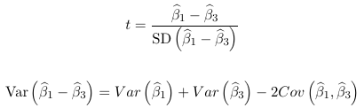
or the Wald test with w = t2. Only variances of coefficients are reported by default in PROC GENMOD, so to get the covariance matrix the covb option is needed in the model statement. But when we want to test more than one linear combination of parameters at the same time this becomes complex and time consuming to do manually.
Within SAS's PROC GENMOD or LOGISTIC we use CONTRAST and ESTIMATE statements to carry out this type of test.
title1 ’ Contrasting <200 vs . 220 -259 with CONTRAST and ESTIMATE statements ’;
proc genmod data = CHD ;
class CHOL SBP ;
model CHD / Total = CHOL SBP / dist = Binomial link = logit ;
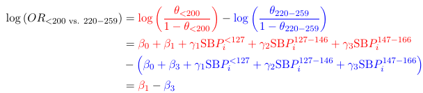
estimate ’ <200 vs . 220 -259 ’ CHOL 0 -1 1 0/ exp ;
contrast ’ <200 vs . 220 -259 ’ CHOL 0 -1 1 0;
run ;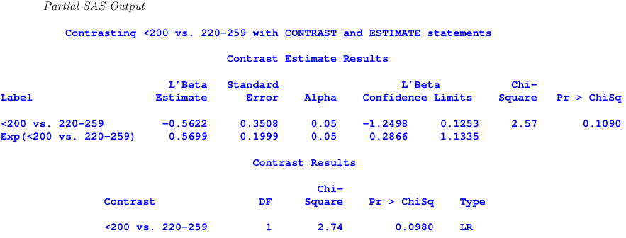
The chi-sqaure test statistic in the two tests is different because estimate uses a t-test while contrast uses a Wald test.
For a categorical variable variable has k levels, the GLM parameterization generates k indicators to
include in the model. For this reason, the GLM parameterization produces a singular model matrix.
Note the following:
- The order of the levels in SAS is critical to outcome.
- The values entered in L, the contrast matrix, must be changed if the parameterization (coding) changes.
- In most procedures the default parameterization is less than the full rank parameterization
- You can alter the default parameterization with the param= option and ordering the levels in the class statement (by using PROC FORMAT)
*Code the categories;
data remission ;
input LLI $ 1 -5
cards ;
8 -12 7 1 1
14 -18 7 1 2
20 -24 6 3 3
26 -32 3 2 4
34 -38 4 3 5
run ;
total remiss grp ;
proc format ;
value $a ’ 8 -12 ’ = ’1 ’ ’ 14 -18 ’= ’2 ’’ 20 -24 ’= ’3 ’ ’ 26 -32 ’= ’4 ’ ’ 34 -38 ’= ’5 ’; run ;

*Here the parameters of interest are the 4th and 5th parameter;
title ’ Default order - Alphanumeric ordering ’;
title2 ’ GLM Coding ’;
ods select classlevels parameterestimates contrasts ;
proc genmod data = remission ;
class LLI ;
model remiss / total = LLI ;
contrast ’ 34 -38 vs . 8 -12 ’ LLI 0 0 0 1 -1;
contrast ’ 34 -38 vs . 8 -12 ’ LLI 0 0 0 1 -1/ wald ;
run ;

*Use format to change the order from 1st to 5th;
title ’ Desired order - Using proc format ’;
title2 ’ GLM Coding ’;
ods select classlevels parameterestimates contrasts ;
proc genmod data = remission ;
format LLI $a .;
class LLI ;
model remiss / total = LLI ;
contrast ’ 34 -38 vs . 8 -12 ’ LLI -1 0 0 0 1;
contrast ’ 34 -38 vs . 8 -12 ’ LLI -1 0 0 0 1/ wald ;
run ;

*We only estimate 4 parameters since the effect of 20-24 is 0 so the 3rd and 4th parameters are of interest;
title ’ Changing Default coding in proc genmod ’;
title2 ’ Change to Reference Coding ’;
ods select classlevels parameterestimates contrasts ;
proc genmod data = remission ;
/* Changed to Reference coding using the ’ param = ref ’ statement . */ ;
class LLI ( ref = ’ 20 -24 ’) / param = ref ;
model remiss / total = LLI ;
contrast ’ 34 -38 vs . 8 -12 ’ LLI 0 0 1 -1;
run ;

*Testing: λ4 − λ5 = λ4 − (−λ1 − λ2 − λ3 − λ4 ) = (1)λ1 + (1)λ2 + (1)λ3 + (2)λ4;
title ’ Changing Default coding in proc genmod ’;
title2 ’ Change to Effect Coding ’;
ods select classlevels parameterestimates contrasts ;
BS853 - Generalized Linear Models
proc genmod data = remission ;
class LLI / param = effect ;
model remiss / total = LLI ;
contrast ’ 34 -38 vs . 8 -12 ’ LLI
run ;

*Comparing the 1st, 4th and 5th parameters;
title1 ’ Two contrasts for multiple hypothesis ’;
ods select pa ra meterestimates contrasts ;
proc genmod data = remission ;
class LLI ;
model remiss / total = LLI ;
contrast ’ 34 -38 vs . 14 -18 vs . 8 -12 ’ LLI 0 0 0 1 -1 , /* ( H01 ) */
LLI 1 0 0 0 -1; /* ( H02 ) */
run ;

*Contrasts involving interactions;
options pageno =1;
title1 ’ OR in each Department for the Saturated Model ’;
ods output estimates = estimates parminfo covB parameterestimates classlevels ;
proc genmod data = one ;
class department SEX ;
model yes / total = SEX | department / link = logit dist = bin covb ;
estimate ’ SEX1 ’ SEX 1 -1 department * SEX 1 -1 0 0 0 0 0 0 0 0 0 0/ exp;
estimate ’ SEX2 ’ SEX 1 -1 department * SEX 0 0 1 -1 0 0 0 0 0 0 0 0/ exp;
estimate ’ SEX3 ’ SEX 1 -1 department * SEX 0 0 0 0 1 -1 0 0 0 0 0 0/ exp;
estimate ’ SEX4 ’ SEX 1 -1 department * SEX 0 0 0 0 0 0 1 -1 0 0 0 0/ exp;
estimate ’ SEX5 ’ SEX 1 -1 department * SEX 0 0 0 0 0 0 0 0 1 -1 0 0/ exp;
estimate ’ SEX6 ’ SEX 1 -1 department * SEX 0 0 0 0 0 0 0 0 0 0 1 -1/ exp;
run ;
Note:
- In PROC LOGISTIC the estimate and contrast statement is implemented exactly the same as above
- If you use the default less-than-full-rank GLM class variable parameterization, each row of the L matrix is checked for estimability. If GENMOD finds a contrast to be non-estimatable it displays missing values in corresponding rows in the results.
- If an effect is not specified in the CONTRAST statement, all of its coefficients in the L matrix are set to 0. If too many values are specified for an effect the extra ones are ignored. If too few are specified, the remaining ones are set to 0.
- For specifying contrasts for interactions, the order you list your categorical variables in the class statement is important
No Comments