GLM for Correlated Data

So far the models we've covered assume independence between observations collected on separate individuals. When observation are correlated models that incorporate the existing correlation in the data should be employed. There are many approaches are proposed but here we focus on Generalized Estimating Equations (GEE) and Mixed Effects Generalized Linear Models.

Generalized Estimating Equations Methods

For classical generalized linear model we assume only one observation was collected per subject with a set of predictors.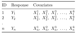

The most common type of correlated data is longitudinal, collected on the same subjects over time. For data with 3 time points: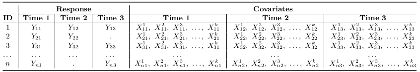

Other examples of correlated data are: Data collected from different locations on the same subject or collected on different subjects which are related.

In SAS the function to estimate GEE models is PROC GENMOD. For normal models it can be fit in other procedures, such as PROC MIXED. Using PROC GENMOD the data must be inputted in long form (multiple observations per subject):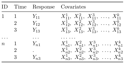

Now we could analyze the data by observing the counts out the outcome while ignoring the correlation between subjects, or simply observe the linear correlation between outcome and time, but in general ignoring the dependency of the observations will in general overestimate the standard errors of the time-dependent predictors since we haven't accounted for within-subject variability.

The influence of correlation on statistical inference can be observed by inspecting its influence on the sample size for a design that collects data repeatedly over time. In comparing 2 groups in terms of means on a measured outcome Y_ij where i is subjects and j is group, and in each group there are m subjects and within each group there are n repeated observations. Further assuming that Var(Y_ij) = σ² and that within each group Cor(Y_ij, Y_hj) = ρ where i != h. Then the sample size needed to detect a difference in means of outcome, d = μ₁ + μ₂ = E(Y_i1) - E(Y_i2) with power P = 1 - Q and type I error (α) is:

$$ m = {{2(z\alpha + zQ)^2\sigma^2(1 + (n - 1)\rho)} \over {nd^2}} = {{2(z\alpha + zQ)^2(1 + (n - 1)\rho)} \over {n\Delta^2}}$$

Where $\Delta = d / \sigma $ is the mean difference in standard deviation units. From the formula, the higher the correlation (ρ) the larger the larger the m.

However, standard errors of the time-independent predictors (such as treatment) will be underestimated. The long form of the data makes it seem like there's 4 times as much data then there really is. In comparing 2 groups in terms of slopes (rate of change) on a measured outcome, the sample size needed to detect a difference in slopes of a predictor x_h and outcome d = β₁ - β₂ with power P = 1 - Q is:

$$ m = {{2(z\alpha + zQ)^2\sigma^2(1 - \rho)} \over {ns^2_xd^2}} $$

Where $ s^2_x = {\sum_j {(x_j \bar x)^2} \over n} $ is the subject variance of the covariate values x_j. From the above formula the higher the correlation (ρ) the smaller the m.

Correlated data are modeled using the same link function and linear predictor setup (systematic component) as in an independent model, the difference being that the covariance structure of the correlated observations are incorporated too.

The strategy is too propose a set of equations (called Generalized Estimating Equations) that replaces the likelihood equations. These equations can then be used to estimate the parameters. The GEE for estimating the parameters β is an extension of the likelihood equations for independent observations to correlated data are:

$$ S(β) = \sum_{i = 1}^K {D'_i V_i^{-1} (Y_i - \mu_i(\beta)) } = 0 $$

where $ D_i = {{\delta\mu_i} \over {\delta\beta}} $ and $g(\mu_i) = X\beta$

The GEE approach accounts for the dependency among observations through the specifications of Vi's. The correction for within subject correlation is incorporated by assuming a priori correlation structure ("working correlation structure") for repeated measurements. SAS has a large number of pre-specified covariance structures built in.

Consider R_i (α) to be the working correlation matrix and assume that this matrix is determined by the parameters α. With this, the variance covariance matrix V_i is calculated as:

$$ V_i = \gamma A^{1/2}R_i(\alpha)A^{1/2} $$

where A is the diagonal matrix given by the variance function evaluated at the means, that is $A_{ii} = V(\mu_i) $and $ \gamma$ is the dispersion parameter

For the classical generalized linear models, the assumed variance-covariance structure for the observation collected on the same subject over 4 time points are:

$$ \begin{bmatrix}
\sigma_{y1}^2 & 0 & 0 & 0\\
0 & \sigma_{y2}^2 & 0 & 0\\
0 & 0 & \sigma_{y3}^2 & 0\\
0 & 0 & 0 & \sigma_{y4}^2
\end{bmatrix} $$

where $\sigma_{y1}^2, \sigma_{y2}^2,\sigma_{y3}^2,\sigma_{y4}^2$ are the correlation of the outcomes at times 1, 2, 3 and 4 respectively. In GEE the assumed variance-covariance structure is allowed to have some values other than 0 off the main diagonal, that is:

$$ \begin{bmatrix}
\sigma_{y1}^2 & v_1 & v_2 & v_3\\
v_1 & \sigma_{y2}^2 & v_4 & v_5\\
v_2 & v_4 & \sigma_{y3}^2 & v_6\\
v_3 & v_5 & v_6 & \sigma_{y4}^2
\end{bmatrix} $$

Where v_j are covariance parameters

Correlation Structure

Assuming we measure the response at 4 follow-up times the above correlation structure can be represented as follows:

Independent (native analysis) - IND
$$ \begin{bmatrix}
1 & 0 & 0 & 0\\
0 & 1 & 0 & 0\\
0 & 0 & 1 & 0\\
0 & 0 & 0 & 1
\end{bmatrix} $$
Exchangeable (compound symmetry) - EXCH or CS
$$ \begin{bmatrix}
1 & \rho & \rho & \rho\\
\rho & 1 & \rho & \rho\\
\rho & \rho & 1 & \rho\\
\rho & \rho & \rho & 1
\end{bmatrix} $$
Auto-regressive - AR(1)
$$ \begin{bmatrix}
1 & \rho & \rho^2 & \rho^3\\
\rho & 1 & \rho & \rho^2\\
\rho^2 & \rho & 1 & \rho\\
\rho^3 & \rho^2 & \rho & 1
\end{bmatrix} $$
M-Dependent - MDEP(2)
$$ \begin{bmatrix}
1 & \rho_1 & \rho_2 & 0\\
\rho_1 & 1 & \rho_1 & \rho_2\\
\rho_2 & \rho_1 & 1 & \rho_1\\
0 & \rho_2 & \rho_1 & 1
\end{bmatrix} $$
Unstructured (no specification) - UN
$$ \begin{bmatrix}
1 & \rho_1 & \rho_2 & \rho_3\\
\rho_1 & 1 & \rho_4 & \rho_5\\
\rho_2 & \rho_4 & 1 & \rho_6\\
\rho_3 & \rho_5 & \rho_6 & 1
\end{bmatrix} $$

And many more. Always choose the simplest structure (that uses the fewest parameters) that fits the data well.

Parameter Estimation Using the Iterative Algorithm

First a native linear regression analysis is carried out, assuming the observations within subject are independent.
The residuals are calculated from the native model (observed-predicted) and the working correlation matrix is estimated from these residuals
The regression coefficients are re-estimated, correcting for the correlation
GOTO Step 2 and repeat until convergence is met

Missing Data

In model fitting the GEE methodology uses the "all available pairs" (pair = Response, set of predictor values), in which all non-missing pairs of data are used in the estimating the working correlation parameters. This approach is not always appropriate (when missing data has a pattern).

Model Selection

The generalized estimating equations (GEE) method is not a likelihood-based method, and thus the classical goodness of fit statistics are not displayed in SAS. The Quasilikihood under the Independence model Criterion (QIC) has been proposed to compare GEE models. QICu is a related statistic that penalized model complexity, defined as:

$$ QICu = QIC + 2p $$

where p is the number of parameters in the model and can be used in model selection. Two models do not need to be nested in order to use QIC or QICu to compare. QIC can be used to select a working correlation structure for a given model while QICu should not. Smaller values of QIC or QICu are indicative of a better model. This was implemented in SAS starting in version 9.2.

Statistical tests based on Wald test statistic method can also be used to test for sequentially adding terms to a model or to compare two nested models.

We can observe the starting correlation structure with PROC CORR in SAS to decide on a starting structure.

*Put data in long format;
proc transpose data=seizures out=wides(where=( col1 ne .));;
  by id;
  var logresponse;
  copy TREATMENT BASELINE AGE;
run;

title1 'Estimated correlation ';
proc corr data=wides;
  var col1-col4;
run;

title1 ' A GEE model with a time independent treatment effect';
title2 ' Exchangeable correlation structure ';
proc genmod data=seizures;
  class  id time treatment; 
  model RESPONSE=TIME TREATMENT BASELINE AGE/d=poisson; 
  repeated subject = id / type=cs corrw; 
  estimate 'TRT 1 vs. 0'  TREATMENT -1 1/exp;
run; 
quit;

Generalized Linear Mixed Models (GLMM)

Generalized linear models for independent data are extensions (generalizations of the classical linear model. The coefficients in the classical generalized linear models do not vary with the subject, they are fixed. We can further extend the classifcal generalized linear model to also allow coefficients that are random (in a way that their value could vary with subject). These effects are classed random effects, thus mixed effects model.

A typical example where this model would be employed is when the data are collected longitudinally on the same subjects. The model for this situation would be represented as:

$$ y_{it} = \alpha_0 + \beta_0*t + \alpha_i + \beta_i*t + \epsilon_{it} $$

where i indexes the subjects and t is the time. The model has fixed effects for intercept (alpha0) and slope of time (beta0) and random effects for the intercept (alpha_i) and slope for time (beta_i. In a way we fit a line for each subject in the study:

$$ y_{it} = (\alpha_0 + \alpha_i) + (\beta_i + \beta_0)*t + \epsilon_{it} $$

Such a model has a lot of parameters. Assumptions that reduces the number of parameters are:

thus reducing the number of parameters to 2 and viewing these 'deviations' as random quantities or random effects. If the two sets of parameters are assumed to co-vary, one can assume that the two effects follow a multivariate normal distribution, or: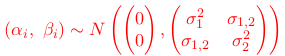

One byproduct of the assumptions above is that observations from the same subjects are correlated. To see this we show that correlation between observations on the same i subjects collected at different time points (t1 and t2) is not 0.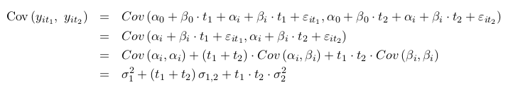

where we used the fact that the errors have mean 0 and are independent of the random effects. For this reason the random effects models are used to model correlated data. The Mixed Effects models are also used for clustered data in general, not only longitudinal data.

The general form of the Linear Mixed Effects Model (LMM) is:

$$ y = X\beta + Z\gamma + \epsilon$$
where y is the dependent variable (outcome), X is the matrix of predictor variables, Z is a design matrix, beta is a vector of fixed effects, gamma is a vector of random effects, and epsilon is a random error which follows a normal distribution with mean 0.

The Generalized Linear Mixed Effects Models (GLMM) extend the LMM by allowing the response variables to follow any distributions from the exponential family (which includes the normal distribution). In addition, a link function is allowed to link the mean of the outcome (mu) to covariates and random effects. The linear predictor in this example includes both the fixed and random effects.

$$ \eta = X\beta + Z\gamma $$

We then assume that $g(\mu) = \eta $

Even though the outcome distribution can be chosen to be different from normal, the distribution of random effects is almost always made to be normal.

We below consider a mixed effects Poisson model with a log link fit to the model with a random intercept and fixed effects for time, treatment, baseline and age.

/***** GLMM Model ***********/
title1 ' A GLMM model with a time independent treatment effect';
proc glimmix data=seizures;
  class  id time treatment; 
  model RESPONSE=TIME TREATMENT BASELINE AGE/ s d=poisson link=log; 
  random intercept /subject = id ; 
  estimate 'TRT 1 vs. 0'  TREATMENT -1 1/exp cl;
run; 
quit;

The results are similar to the results from GEE. But the two do differ as they are different models. In terms of the interpretation of the coefficients, there is a difference in the case of non-linear models. One difference between GEE and GLM is that GEE estimates population-average while GLMM is the subject-specific effect. These are the same in linear models, but not in non-linear as above.