GLM for Count Data
Generalized linear models for count data are regression techniques available for modeling outcomes describing a type of discrete data where the occurrence might be relatively rare. A common distribution for such a random variable is Poisson.
The probability that a variable Y with a Poisson distribution is equal to a count value
$${ P(Y = y) = {{\lambda^y e^{-\lambda}} \over {y!}}} y = 0, 1, 2, ..., \infty $$
where λ is the average count called the rate
The Poisson distribution has a mean which is equal to the variance:
E(Y) = Var(Y) = \(\lambda\)
The mean number of events is the rate of incidence multiplied by time passed
Because of this assumption, the Poisson distribution also has the following properties:
- If Y_1 ~ Poisson(λ_1) and Y_2 ~ Poisson(λ_2) where Y_1 and Y_2 are the number of subjects in groups 1 and 2, then Y_1 + Y_2 ~ Poisson(λ_1 + λ_2)
- This generalizes to the situation of n groups as: Assuming n independent counts of Y_i are measured, if each Y_i has the same expected number of events λ then Y_1 + Y_2 + ... + Y_n ~ Poisson(nλ). In this situation λ is interpretable as the average number of events per group.
Poisson Regression as a GLM
To specify a generalized linear model we need (1) the distribution of outcome, (2) the link function, and (3) the variance function. For Poisson regression these are (1) Poisson, (2) Log, and (3) identity.
Let's consider a binomial example from a previous class where:
$$ Y_{ij} \approx Binomial(N_{ij}, λ_{ij}) $$
Given a variable Y ~ Binomial(n, p), where n is number of experiments and p the probability of success, this binomial distribution can be approximated well by the Poisson distribution with mean n*p.
So from that we can assume the distribution of Y also follows:
$$ Y_{ij} \approx Poisson(N_{ij} λ_{ij}) $$
and thus
$$ log(E(Y_{ij})) = log(N_{ij}) + log(\lambda_{ij}) $$
Since log(N_ij) is calculated from the data, we will proceed by modeling log(λ_ij) as a linear combination of the predictors:
$$ log{λ_{ij} } = μ + β_1X_{ij}^1 + β_2 X_{ij}^2 + . . . + β_k X_{ij}^k $$
The natural log is attractive as a link function for several reasons:
- The log link maps relative rates into additive effects
- With this link, parameters are readily interpretable as rate ratios, these ratios are called relative risks (risk ratios)
- The log link transforms positive values into the whole real link.
This the Poisson regression models extend the loglinear models; loglinear models are instances of Poisson regression.
Modeling Details
With the assumption
$$ E(Y_i) = N_i*λ_i $$
then using a log link we have:
$$ log(E(Y_{i})) = log(N_{i}) + log(\lambda_{i}) $$
Assuming we have a set of k predictors X1, X2, ..., Xk (continuous and/or ordinal and/or nominal), in Poisson regression one the linear predictors can be represented as:
$$ log{λ_i} = μ + β_1X_{i}^1 + β_2 X_{i}^2 + . . . + β_k X_{i}^k $$
We can represent the expected value as: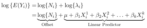
Where the term log(N_i) is called the offset. The offfset allows us to consider groups of different sizes in the model, but carries little value in terms of outcome.
In SAS we can use GENMOD to specify the Poisson distribution and an optional offset, but we must calculate the value ourselves.
proc genmod data = claims ;
class district car age ;
model C = district car age / offset = logN dist = poisson link = log obstats ;
estimate ’ district 1 vs . 4 ’ district 1 0 0 -1/ exp ;
run ;
In the results, the distribution of the chi-squared residuals (or deviance residuals) can be approximated by standard normal distribution. When the number of cells is large this assumption can be checked via a normal quantile plot, such as PROC UNIVARIATE; A linear pattern is evidence of a good fit.
Interpretation of Parameters
Interpretation is much the same as in a binomial model, we compare the rate of incidence in the reference group to that of the other groups:
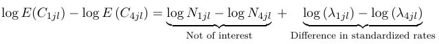
The most common use of a Poisson regression is in the analysis of time-to-event or survival. In cohort studies, the analysis of data usually involves estimation of disease during a defined period of observation; In this case the denominator of such a rate is measured in years of observation per person (person-years).
Over-dispersion in Poisson Regression
Over-dispersion occurs when the variance of the response exceeds the mean (nominal variance in Poisson); That is:
$$ var(Y) > E(Y) = n \pi (1 - \pi) $$; Where n is the number of trials and π is the probability of success
This can be the result of several phenomena:
- When the response is a random sum of independent variables, that is Y = R_1 + R_2 + ... + R_k where k is distributed as Poisson independent of R_i's
- When Y ~ Poisson(L), where L is random (this appears when there is inter-subject variability). The classical assumption is that L ~ Gamma(α, μ)
- When missing important covariates
- When the total population (N) is random rather than fixed
Regardless of the source of over-dispersion, methods that take the over-dispersion into account should not be used. Not taking into account the over-dispersion results in many false positive test results, as without taking into account the over-dispersion the estimates for the variability of the coefficients underestimates the scale of w.
We can use a generic method to model the over-dispersion by modifying the variance function from the identity function g(λ) = λ to g(λ) = w2λ. w is called the scale or over-dispersion parameter.
An estimator for w is:
$$ w^2 = {X^2 \over {n-p}}= { \sum_i {(n_i - \hat m_i)^2 \over \hat m_i} \over {n-p} }$$
Where p is the number of parameters and n is the number of observations. If w > 1 we say there is over-dispersion. A similar estimate might be obtained by replacing the Pearson chi-square statistic with the Deviance statistic. One can test for over-dispersion using the Negative Binomial Generalized Linear Model.
Testing for Over-Dispersion in Poisson - Negative Binomial Regression
Scaled deviance and scaled Pearson Chi-Squared can be used to detect over-dispersion or under-dispersion in the Poisson regression. We can test for over-dispersion by comparing deviances from a generalized linear model based on Poisson distribution assumption for the outcomes with log link and offset and a generalized linear model based on the negative binomial distribution assumption for the outcome with a log link and offset.
For a negative binomial distribution: var(Y) = E(Y) + k{E(Y)}2
Where k >= 0 (the negative binomial likelihood reduces to Poisson when k = 0)
In testing over-dispersion in a Poisson regression the hypotheses are: H0: k=0 vs Ha: k > 0
The negative binomial regression can be fit in SAS as the Poisson regression, with the change that in the dist option we specify 'NB'.
To carry out the test:
- Run a Poisson Regression
- Run the Negative Binomial
- Subtract the log-likelihood values from teh negative binomial regression and Poisson regression and multiply by 2 to obtain the test statistic
O = 2 * (LL(Negative Binomial) - LL(Poisson)) - If the test significance level is α, compare it against a critical value from a Chi-Square distributino with one degree of freedom and level 2α
title2 ’ Using GENMOD - Poisson Regression ’;
ods select Modelfit ;
proc genmod data = incidence ;
class age race ;
model cases = age race / dist = poisson link = log offset = logT ;
run ;

title2 ’ Using GENMOD - Negative Binomial Regression ’;
proc genmod data = incidence ;
class age race ;
model cases = age race / dist = NB link = log offset = logT ;
run ;
Note: Under-dispersion cannot be tested with this method.
Zero-Inflated Poisson
Zero-Inflated Poisson (ZIP) and Negative-Binomial Models deal with situations where there is an added number of instances of data with a count of 0. Zero-inflated models have become fairly popular and have been implemented in many statistical packages.
The ZIP model is one way to allow for over-dispersion with Poisson data. The model assumes that the data values come from a mixture of two top distributions: one set of counts from a standard Poisson distribution, and the other that generates zero counts with probability 1. The value 0 could come from either of the two distributions. A Bernoulli generalized linear model can be used to predict which group an individual belongs to: the one in which the values come from the distribution that only generates 0 counts or from one that follows a Poisson distribution.
The ZIP can be thought of as a latent class model. The assumption being that there exists a Bernoulli (unobserved) variable Z that indicates whether the count comes from the certain 0 distribution or from a Poisson distribution. First remember that for a Poisson variable Y:
$${ P(Y = y) = {{\lambda^y e^{-\lambda}} \over {y!}}} $$
and thus:
$$ P(Y = 0) = {{ e^{-\lambda}}} $$
For an individual i, Zi = 1 then the count will be 0, while if Zi = 0 then the count comes from the Poisson distribution. If P(Zi = 1) = \(\pi_i\) then:
$$ P(Y_i = 0 | X_i) = \pi_i + (1 - \pi_i) P(0|X_i) = \pi_i + (1 - \pi_i) e^{ -\lambda_i } $$
$$ P(Y_i = y | X_i) = (1 - \pi_i)P(y | X_i) =(1 - \pi_i) {{\lambda^y e^{-\lambda}} \over {y!}} $$ for y > 0
The mean of this variable:
$$ E(Y_i | X_i) = (0 * \pi_i) + \lambda_i (1 - \pi_i) = \lambda_i (1-\pi_i) $$
The variance is:
$$ Var(Y_i | X_i) = \lambda_i (1 - \pi_i) (1 + \lambda_i \pi_i) $$
Noting that Var(Yi | Xi) > E(Yi | Xi), so the variance is larger than a Poisson variance.
One can then proceed by modeling both the parameter π (mixture probability) and the parameter λ (the mean of the Poisson count) as a function of the covariates by first transforming these parameter values using link functions.
Often a logit link is used for the π and a log link for λ. In other words the model assumes:
- For the π parameter assume the identity
\( log( {\pi_i \over {( 1 - \pi_i) }} ) = \gamma X_i \) - For the λ parameter assume the identity
log(λi) = β Zi
The covariates in the model for π can be different or the same as the covariates in the model for λs. A Zero-Inflated negative binomial (ZINB) can be defined similarly.
In cases with excess 0's the ZIP model usually fits better than a Poisson generalized linear model. Often, a negative Binomial model fits well with data that has excess of zeros. The ZINB model fits better than a conventional Negative Binomial model regression model if the data present with both over-dispersion and excess of zeros.
title1 ’ Zero Inflated Poisson Regression ( Model 7) ’;
proc genmod data = absences ;
class C S A L / param = ref ;
model days = C | A | S | L @2 / dist = zip ;
zeromodel C S / link = logit ;
run ;
The interpretation of parameters for the above model is complex because of the presence of three two-way interactions, but the steps involved would follow the interpretation in the Poisson regression model.
No Comments