Survival Analysis in Clinical Trials
We've already covered survival analysis in great detail here. This will be review, application to clinical trials, and SAS implementation.
Survival analysis uses class methods of studying occurrence and time of events; it was traditionally designed to study death, but can be used with any type of time to event outcome. These are special cases when a t-test is not appropriate; as the data is skewed and there are values that need to be censored before the end of study.
Participants enter the study event-free and the outcome is to assess if and when the event occurred. We can then investigate if the event occurs differently in other groups. Patients are typically randomized at different dates in the recruitment period and time is measured on a continuous scale. We measure time in the study as the time between randomization and either the patient:
- Has the event (Failure time)
- Is last measured in the study and does not have the event (Censoring time)
Right Censoring
Most common form of censoring and the ideal scenario; Participants are followed for a time but the event of interest does not occur. All we know is that the time of the event is greater than a certain value but it is unknown by how much.
- End of study
- Loss to follow-up (withdrawal or dis-enrollment)
- A completing risk - A different event that occurs and makes it impossible to determine when the event of interest occurs
Interval Censoring
The time for an event occurs between two time points in the study but the investigators do not know the exact date. This could occur when the outcome is self-reported at 3 month intervals, for example. There are special methods for interval censoring in SAS we will not cover here (PROC ICLIFETEST)
The Survival Function
The survival function S(t) is a mathematical function that represents the probability of surviving beyond a particular time t. We can plot the % surviving (without event) on the Y-axis and time on the X-axis to see when most of the events occurred.
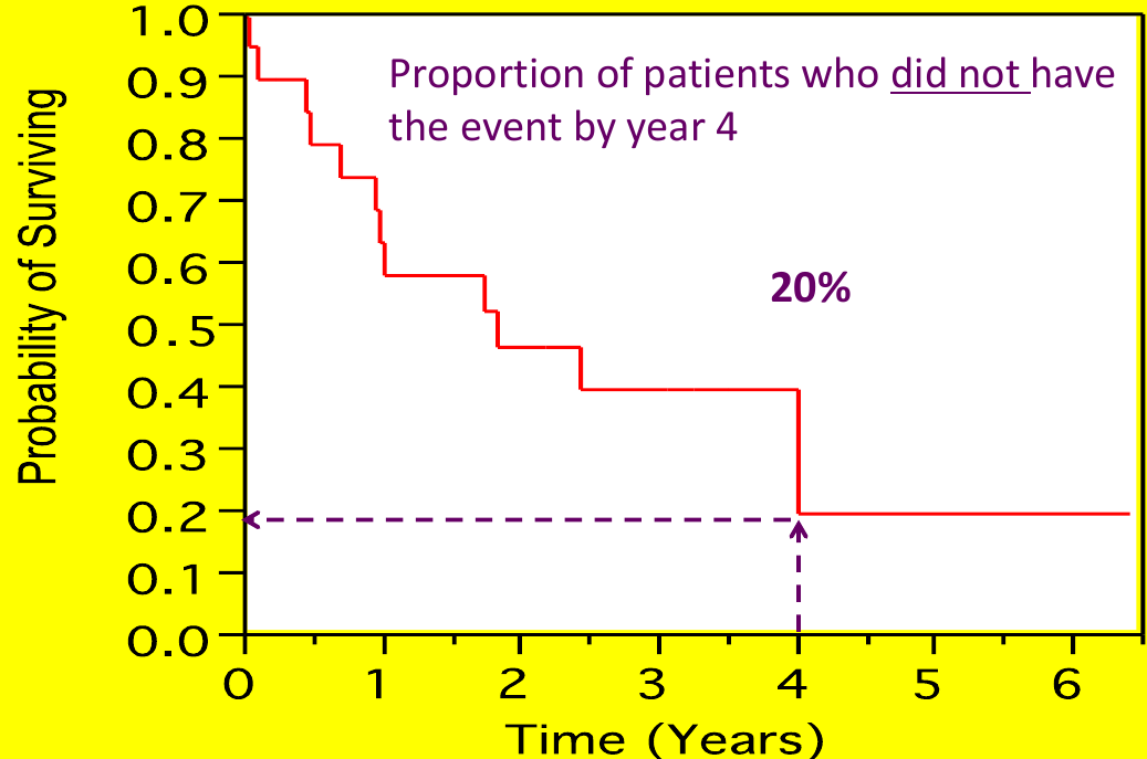
Each step is an "event", but cesnroing events are often marked as an 'X' (no step)
The most commonly used method for estimation of the survival function is the Kaplan-Meier (or product-limit estimator). Suppose there are k distinct event times and n subjects at risk of event, with dj subjects with outcome at time tj: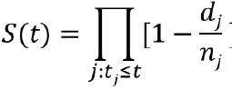
We can visualize this in a chart: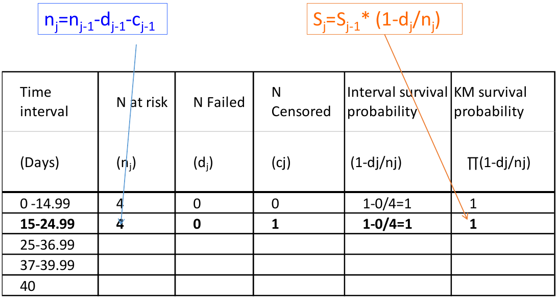
Kaplan-Meier estimates are calculated from the conditional probability of experiencing the event
P(A, B, C) = P(C | A, B)*P(B|A)*P(A)
Ex. S(37) -> Survival estimate at day 37 = P(T > 37 & T > 25 & T > 15) -> Probability of surviving past day 37, 25 and 15
* Computes tables of survival estimates, KM survival curves and log-rank test;
proc lifetest data=mysurv;
time time*cvd_death(0);
strata treat;
run;
Above cvd_death is the name of the event/censoring variable, and the strata is what we want to compare survival. 
In the above sample output:
- "Survival" Represents the KM survival estimate
- "Failure" is the cumulative probability of the event (1 - KM probability).
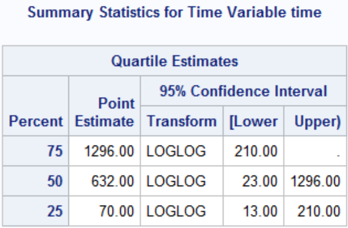
The quartile estimates Point Estimate gives the smallest event time such that the probability of event is greater than [.25/.5/.75]. There may not be a point estimate if the number of observed events/Failure never reached the percent.
Comparing Survival Curves
Are the curves similar? At what point do they diverge? When do most events occur?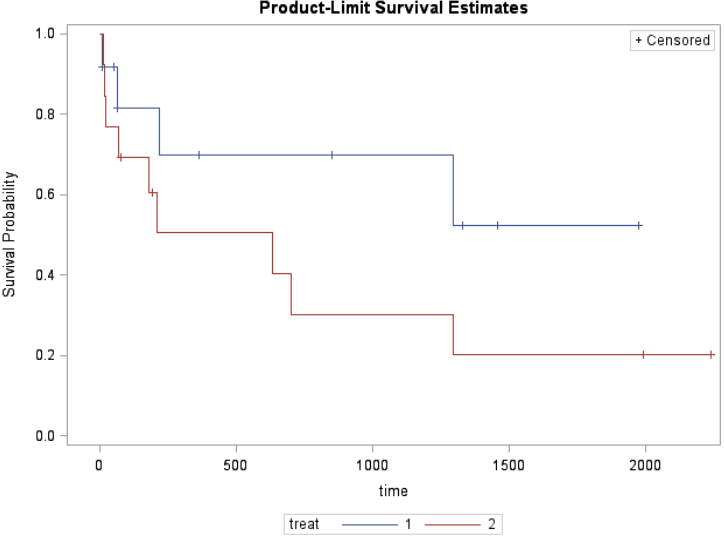
H0: No difference in survival between treatments (KM survival curves are the same)
HA: Difference in survival between treatments (KM survival curves are the different)
![]()
Where r is the number of event times d1j is the number of events in group 1 at time j and eij is the expected number of events in group 1 at time j.
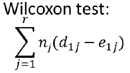
Where nj is number of individuals at risk at each time point (Weighted sum); Gives more weight to early times than later times
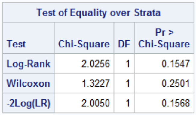
Both log-rank and Wilcoxon test follow a chi-square distribution with 1 df (if G treatments then df = G - 1)
Assumption: Non-Informative Censoring
We assume all individuals who are censored have the same risk of the event (or prognosis) as those who remain in the study (conditional on explanatory variables). There is no statistical test for informative censoring, we just need to adjust estimates for variables that are likely to affect the rate of censoring (need regression models).
Ex. The outcome is death and very sick subjects are less likely to attend study visits.
Comparing Treatments
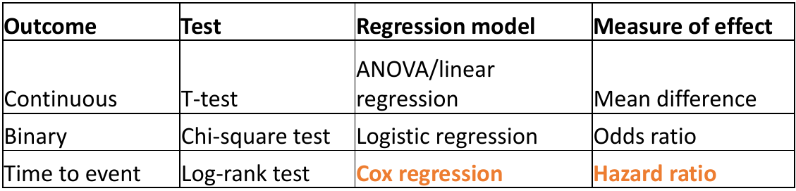
The Hazard (or hazard rate) is the instantaneous risk/rate of experiencing the event at time t. It is not a risk.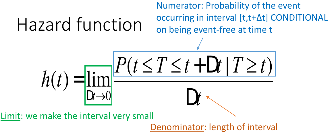
Interpretation: "The hazard of event for the new treatment is 44% of the hazard of the active control group. The 95% CI contains 1 so it is not significant."
In the Cox Proportional Hazards Regression we create dummy variables fro the treatment group: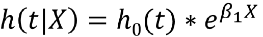
Which can be expressed as:![]()
HR<1 (or β<0): lower hazard of the event compared to reference group
HR>1 (or β>0): larger hazard of the event compared to reference group
Proportional Hazards assumption must be met for a Cox model. That is the separate treatment plots of ln(-ln(S(t)) vs t should be parallel.
Also we can adjust for covariates just like in proc glm ANOVA where we assess interaction and factors.
*Cox Model;
proc phreg data=mysurv;
class treat (param=ref ref='2');
model time*cvd_death(0)=
treat/risklimits;
run;

*Log-log survival plot;
proc lifetest data=mysurv plots=(loglogs);
time time*cvdmort(0);
strata treat;
run;
Partial Likelihood
The LR function for Cox models can be factored into
- One part that depends on h0t and β
- The other part that depends on β alone (partial likelihood)
- We treat the partial likelihood as an ordinary likelihood:
• Estimate values of β that maximize partial likelihood
• Asymptotically consistent and normally distributed
• Estimates are (only slightly) less efficient
No Comments