Continuous and Binary Endpoints

Outcomes are either continuous or dichotomous. Primary and secondary outcomes must be defined a priori in the protocol. The sample size for the study is based on the primary outcome.

When determining if a clinical trial is effective we test a hypothesis of a primary outcome, and we may have several secondary outcomes which are more exploratory. We can't define many outcomes and pick the most successful, it would be like rolling dice many times; It increases the chance of type 1 error (rejecting the null hypothesis when it is true). One could also adjust the p-value/type one error rate to account for multiple testing, but more on this later.

When relevant to the study continuous variable can be coded as a binary one, but leads to a loss of information.

Binary Outcomes Measures

We determine if two or more treatments differ significantly with respect to the "risk" of the outcome (called the event rate)

1 divided by the risk difference (event rate difference in control and treatment) is called the number needed to treat. It is interpreted as "you need to treat X people to prevent one event"

The event rate in the treatment group divided by the event rate in the placebo group is called the Relative Risk.

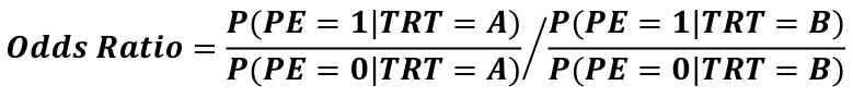
Statisticians really like odds ratios because they translate really nicely to logistic regressions.

Statistical Analysis of Randomized Controlled Trials (RCT)

Define outcome <- Statistical Analysis plan/protocol
- Binary, continuous, etc.
State the null hypothesis
- One or two sided; alpha level
Descriptive statistics <- Data Analysis
Determine appropriate statistical test
Parameter estimates, confidence interval, p-value
Write conclusions

Superiority Trial - We expect that the new treatment is better than the control
H₀: μ_A = μ_B
H_A: μ_A != μ_B

Note that we test the hypothesis two sided even though we think the effect will be one-directional. This is an FDA recommendation, one sided tests are allowed but use .025 level of significance. Two sided tests require larger samples size than one sided at alpha level .05.

Writing Conclusions

Statistical Methodology Section

The primary outcome being tested
Describe tests used, assumptions, and groups tested

Reporting of Results

Mean and confidence intervals
Test statistic values
Reject or accept the null hypothesis

SAS

Generally we only need to specify a single test, but each test has its own assumptions

Parametric Tests

Parametric tests require the assumption of independence, equal variance and normality. When these assumptions do not hold, try either transformation or non-parametric tests.

We can get the same information from all the following procedures, but there are different options and defaults for each method
PROC TTEST, PROC GLM, PROC REG, PROC ANOVA

PROC TTEST

Test difference between means, and differences in variances via an F-Test

proc ttest data=dbp;
    class trt;
    var diff;
run;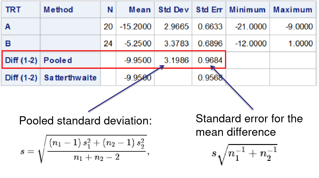

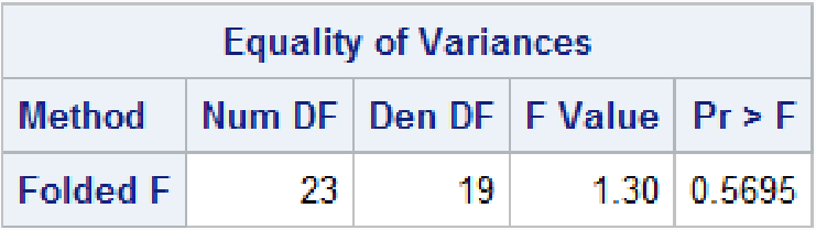
Welch's T-Test can be used if treatment groups have different variance

Proc Reg

Note, when using PROC REG or GLM always put a quit statement at the end or SAS will run forever.

Below we create a dummy variable for the treatment type.

data dbp;
	set dbp;
	if trt='A' then x=1;
	else x=0;
run;
proc reg data=dbp;
	model diff = x;
run; quit;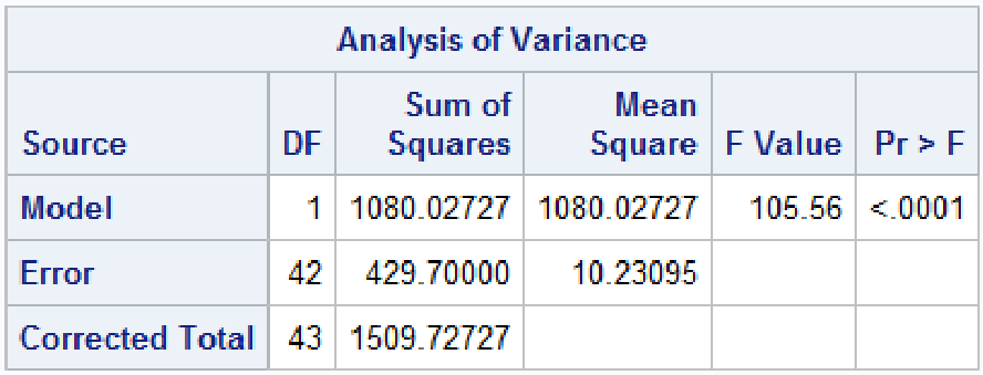

The F statistic is exactly the same p-value and square of the t-test under the assumption of equal variances

Proc GLM

Almost the same as PROC REG but no need for dummy variables

proc glm data=dbp;
	class trt;
	model diff=TRT /solution clparm;
	means TRT/hovtest=levene welch;
run;quit;

Non-Parametric Tests for Two Groups

Non-parametric groups only pay a very small penalty, if the data is normally distributed the test is ~95% as powerful as a ttest

Non-parametric Tests
PROC NPAR1WAY, PROC SURVEYSELECT

Wilcoxon Rank-Sum Test

Works very well on skewed data

proc npar1way data=dbp wilcoxon;
	class TRT;
	var diff;
	*exact wilcoxon; /* request for exact p-value - may take a while */
run;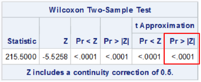

The highlighted is the two sided z test typically reported

Transforming Data

Natural logarithmic transformations are the most widely used in health data, where data often follows a log-normal distribution. Can only be used with positive values.

Running a t-test may not lead to an equivalent null hypothesis if the variances of the two groups are different

data dbp;
	set dbp;
	logAge=log(Age);
run;
proc univariate
	data=dbp;
	class TRT;
	histogram;
	var Age logAge;
run;

Bootstrap Confidence Intervals

How they work:

Compute statistics of interest for the original data
Resample B times from the data with replacement to form B bootstrap samples
Compute statistics of interest on each bootstrap sample
- this creates the bootstrap distribution which approximates the sampling distribution
Use the bootstrap distribution to obtain estimates such as confidence interval and standard error

/* 1. Compute statistics in the original data */
proc means data=new;
class trt;
var diff;
run;
/* 2. Bootstrap resampling */
proc surveyselect data=new noprint seed=1
out=BootSSFreq(rename=(Replicate=B))
method=urs /* resample with replacement */
samprate=1 /* each bootstrap sample has N observations */
/* OUTHITS */ /* option to suppress the frequency var */
reps=1000; /* generate 1000 bootstrap resamples */
run;
/* 3. Compute mean for each TRT group and bootstrap sample */
proc means data=BootSSFreq noprint;
class TRT;
by B;
freq NumberHits;
var diff;
output out=OutStats; /* approx sampling distribution */
run;
/* 4. Bootstrap distribution and confidence interval */
data boot_mean (keep=B diff TRT);
set OutStats ;
where _STAT_='MEAN' and _TYPE_=1;
run;
proc univariate data=boot_mean noprint;
class TRT;
histogram;
var diff;
output out=boot_ci pctlpre=boot_95CI_ pctlpts=2.5 97.5
pctlname=Lower Upper;
run;
proc print data=boot_ci noobs;
title "Bootstrap confidence intervals";
run; title;