Multiple Comparisons
There are some situations where it may be necessary to have multiple hypothesis tests; ANOVA with more than 2 tables, genetic data, interim analysis, multiple outcomes, etc. Often times clinical trials may have 3 or more arms to reduce administrative burden and improve efficiency and comparability.
Recall hypothesis tests are a way to determine the truth about 2 states and 2 possible outcomes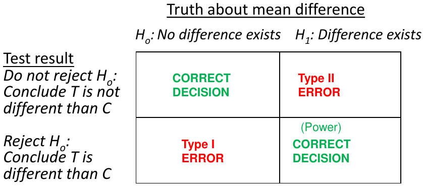
α = probability of a Type 1 error; β = probability of a Type 2 error; 1 - β = power
Assume we carry out m independent statistical tests with significance level α, this means the probability of not making a Type 1 error in any test is: (1-α)*(1-α)*(1-α)*...*(1-α)=(1-α)m
Multiplicity may occur when we use more complex designs, such as 3 or more treatment groups, multiple outcomes, or repeated measurements on the same outcome.
Types of Error Rates
- Comparison-wise Error Rate (CER)
- Type 1 error rate for each comparison
- Family-wise (FWER) or experiment-wise error rate
- Type 1 error rate for the entire group of comparisons
Analytic Strategies
- Define success as "all-or-nothing"
- All tests must be significant
- Ex. Back to Health study where there were two endpoints (a questionnaire and a visual analog scale of pain) the study was only a success when both endpoints showed that yoga was non-inferior to physical therapy for chronic lower back pain.
- This method does not inflate the FWER
- Define success as "either-or" and adjust for multiplicity
- At least one test is significant
- Ex. A burn treatment that could speed up healing or reduce scarring but we are not sure which.
- If both nulls are true the FWER is inflated can be ~ .1
- Use a composite endpoint
- Combining multiple clinical outcomes into a single variable
- Only one test to perform
- No inflation of the FWER
Adjusting for Multiplicity
- Single Step Procedures
- Test each null hypothesis independently of the other hypotheses, order is not important.
- Bonferroni, Tukey, Dunnett
- Stepwise procedures
- Testing is done is a sequence
- Data-driven ordering - The testing sequence is not specified at proir and the hypotheses are tested in order of significance/p-value
- Pre-specified hypothesis ordering - The hypotheses are tested in a pre-specified order
- Holm, Fixed-sequence
- Other multiple comparison procedures:
- Fisher's Least Significant Differences (LSD) - no alpha adjustment
Fisher's Least Significant Differences
We complete the global ANOVA first, if it rejected we simply complete the pairwise comparisons and do not correct the p-values. Easiest method, but this requires the global ANOVA is rejected. The FWER is only controlled when all null hypotheses are true.
proc glm data=headache;
class group;
model outcome=group;
lsmeans group / tdiff pdiff stderr cl;
* tdiff = t-statistics and p-values for pairwise tests;
* pdiff = p-values for pairwise tests;
* stderr = standard errors for means;
* cl = confidence limits;
run;quit;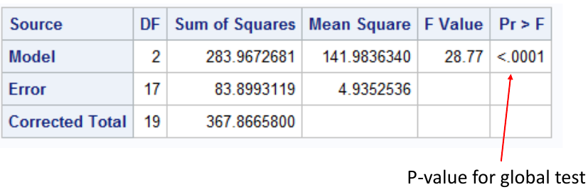
This output suggests we reject the null hypothesis and conclude the mean is different in at least one group. Thus we can do the rest of the pairwise comparisons: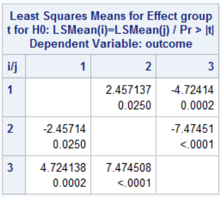
P-Value (Single Step) Adjustments
To correct the comparison-wise alpha level to allow the family-wise comparison level to be controlled at .05. For example, there are two ways to implement the Bonferroni correction:
- Divide the comparison-wise alpha level by the number of comparison and use that as the threshold
- Multiply the observed p-values by the number of comparisons and compare to .05
* Bonferroni correction;
proc glm data=headache;
class group;
model outcome=group;
lsmeans group / tdiff pdiff stderr cl adjust=bon;
run;
quit;

* We can also use Bonferroni correction
with a control group;
proc glm data=headache;
class group;
model outcome=group;
lsmeans group / tdiff
pdiff=control(‘Placebo’) stderr cl
adjust=bon;
run;
quit;

* Tukey-Kramer correction;
proc glm data=headache;
class group;
model outcome=group;
lsmeans group / tdiff pdiff stderr cl adjust=tukey;
run;
quit;

* Dunnett;
proc glm data=headache;
class group;
model outcome=group;
lsmeans group / tdiff
pdiff=control(‘Placebo’) stderr cl
adjust=dunnett;
run;
quit;
The Dunnett's test takes advantage of correlations among test statistics, generally less conservative than Bonferroni (lower Type 2 error rate).
Step-Wise Adjustments
- Holm step-down algorithm (AKA "Stepdown Bonferroni")
- Rank the P-values from smallest to largest along with the null hypotheses
- Step 1: Reject H0_1 if p1 <= α/m, if its rejected go to step 2 otherwise stop and do not reject any further hypotheses.
- Step i = 2, ..., m-1: Reject H0_i if pi <= α/(m-i+1). If H0_i is rejected go to step i + 1 otherwise stop and do not reject any remaining hypotheses
- Step m: Reject H0_m if pm <= α
data pvals;
input test $ raw_p @@;
cards;
AvP 0.0002 NvP 0.0001 NvA 0.025
run;
proc multtest pdata=pvals bonferroni holm out=adjp;
run;- Fixed-sequence procedure
- Suppose there is a natural ordering of the null hypotheses (such as clinical importance) fixed in advance
- The fixed-sequence procedure performs the tests in order without an adjustment for multiplicity as long as all the preceding tests had significant results
- It's the same process as above, do not reject any remaining hypotheses once H0_j is rejected
The FWER is controlled because a hypothesis is tested conditionally on having rejected all the hypotheses that came previously.
No Comments