Baseline Variable Adjustment
Baseline covariates are variables expected to influence the outcome, measured before the start of the intervention. They should describe the population enrolled in the study (Table 1 in all RCT papers). We need to decide what variables to measure, if the groups are comparable, and analyze the interactions and possible confounders.
Post-Randomization variables are collected after randomization. For the purpose of estimating treatment effect we never adjust for post-randomization covariates. Post-randomization variables are crucial for er-protocol effect estimation, mediation, and certain types of trials with adaptive design.
Adjusting for Baseline Imbalance
Conditional Methods included regression models, stratification, propensity score, etc.
Marginal Methods inverse probability weighting, standardization, double robust estimation, etc.
So we know randomization around averages produces balance between groups with respect to all measured and unmeasured factors that may influence outcome. However, this does not guarantee balance in any specific trial for any specific variable. Imbalance is common in trials with small sample size, the rule of thumb is the likelihood of baseline is small when n > 200.
If the treatment groups differ in baseline characteristics any difference in the outcome between group might be due to the difference in characteristics.
The best place to address baseline imbalance is in the design stage by creating a proper randomization strategy. In modern statistics, we can also adjust baseline covariates during the analysis stage.
Assessing Imbalance
Identify covariates expected to have an important influence on the primary outcome and specify how to account for them in the analysis in order to improve precision and to compensate for lack of balance between groups.
Statistical testing is controversial for multiple reasons: multiple testing, its hard to reject the null in small trials and the philosophical problem of type I & II errors. However, the p-value can be adjusted to identify imbalances in baseline by choosing a larger cut-off. There is additional controversy over whether to include p-value in "Table 1".
Stratification can sometimes be used to adjust for factors to improve precision of the treatment effect estimate.
We can assess imbalance through ANOVA output from proc glm in sas:
proc glm data=myzinc;
class zinc (ref='0') female (ref='0') heavy (ref='0') ;
where month=18;
model score_v=zinc female heavy/solution clparm;
run;quit;
The F-test of the model in the output is a test that any one of the predictors is significantly associated with the outcome (not very useful)
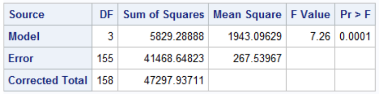
F = MS_model / MS_error
In the sum of squares table we can test whether adding new variables improves model fit:
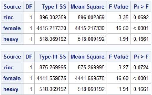
Note that Type I Sum of Squares is cumulative SS if we added the predictors from top to bottom. In Type III sum of sqaures every predictor is adjusted for every other predictor, it is much more widely used.
Analysis of Covariance (ANCOVA)
When an outcome is continuous, adjusting for a baseline covariate that is correlated with the primary outcome can improve precision of treatment effect estimates. Differences between outcome values which can be attributed to differences in the baseline covariate can be removed, leading to more precise estimates.
- The amount of precision gained depends on the strength of the correlation
- Adjusting for variables that are not correlated with the outcome will decrease precision
- Modeling the outcome at the end of the study should be equivalent to the change in outcome between the study end and baseline
proc glm data=myzinc;
class zinc (ref='0') female (ref='0') heavy (ref='0') ;
where month=18;
model score_v=zinc score_v_0 female heavy/solution
clparm;
run;quit;
Binary Outcomes
Instead of average treatment effect we can define a binary variable and use a logistic function to get the odds ratio and other magnitude of effect measures. If the covariate is strongly correlated with outcome then this adjustment will usually lose precision.
data myzinc;
set myzinc;
lower_score=0;
if score_v<score_v_0 then lower_score=1;
run;

proc logistic data=myzinc;
where month=18;
class zinc (ref='0') female (ref='0') heavy (ref='0') ;
model lower_score(event='1')=zinc female heavy /risklimits;
run;
Inverse Probability Weighting (IPW)
- Each individual receives a weight equal to the inverse (reciprocal) of the probability of being assigned to the treatment they received conditional on their baseline covariates L.
Wi = 1 / P(A=a | L) - Fit an adjusted model in the weighted population
- This final model is not conditional on L
- Adjustment for baseline covariates is achieved through weighting where the weights are computed in step 1
- Confidence intervals must be based on robust or bootstrap standard error
*** Step 1: Compute the propensity score (ie
* probability of treatment assignment conditional
* on baseline covariates);
proc logistic data = myzinc;
ods exclude ClassLevelInfo ModelAnova
Association FitStatistics GlobalTests;
class female (ref='0') heavy (ref='0') ;
where month=18;
model zinc(event='1') = female heavy
score_v_0 ;
output out=est_prob p=p_zinc;
run;quit;

*** Step 2: Compute inverse probability weights;
data est_prob;
set est_prob;
if zinc=1 then wt= 1/p_zinc;
else if zinc=0 then wt= 1/(1-p_zinc);

*** Step 3: estimate treatment effect in the weighted
population;
proc genmod data=est_prob;
class id;
weight wt;
model score_v= zinc;
estimate ‘Zinc' intercept 1 zinc 1;
estimate 'Placebo' intercept 1 zinc 0;
repeated subject=id / type=ind;
run;quit;
Disadvantages:
- Relies on assumption of correct model specification
- Typically less efficient than regression adjustment and leads to wider confidence intervals
No Comments