Bayesian Linear Regression

By now we know what a linear regression looks like. Let's consider a special case where number of parameters, p = 0: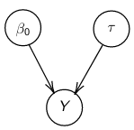

Assume Y is distributed as a normal distribution with mean β₀:
Y|β₀, τ ∼ N(β₀, σ² = 1/τ )

τ = 1 / σ² , also called precision <- Be aware this will be used interchangeably with variance

The density function is: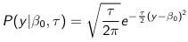

Mean and variance:
E(Y) = μ₀; V(Y) = 1/τ₀ + τ

The Posterior Distribution for β₀ is calculated using Bayes' Theorem

When Mean and Variance are Unknown

We use a Normal prior distribution for the mean β₀ ∼ N(μ₀, τ₀) and a Gamma prior distribution for the precision parameter: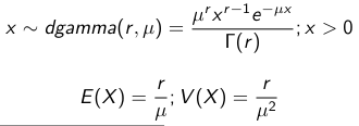

JAGS example:

model.1 <- "model {
	for (i in 1:N) {
		hbf[i] ~ dnorm(b.0,tau.t)
	}
	## prior on precision parameters
	tau.t ~ dgamma(1,1);
	### prior on mean given precision
	mu.0 <- 5
	tau.0 <- 0.44
	b.0 ~ dnorm(mu.0, tau.0);
    
    ### prediction
	hbf.new ~ dnorm(b.0,tau.t)
	pred <- step(hbf.new-20) # hbf >= 20
}"

Predictive Distributions

Given the Prior and Observed data we can compute the probability of a new observation will be greater or less than some integer threshold. The predictive distribution is a distribution of unobserved y^~, that is: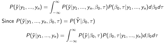

The two sources of variability in prediction are in the parameters V(β₀, τ | y) and the variability in the new observation V(y | β₀, τ)

To simulate from predictive density, do repeatedly:
1. Sample one sample β₀^*, τ* from posterior β₀, τ | y
2. Sample one y^~ ~ N(β₀^*, 1/τ* )
During the Gibbs sampling we generate samples values from the posterior distribution β₀, τ | y
So Generating y^~ ~ N(β₀, τ | y) will produce the correct predictive distribution samples. P(y^~ > 20 | data) is the proportion of y^~ > 20

Log Normal Distributions

Since in the example above the outcome distribution can only be positive we can use a Log-Normal distribution, a continuous distribution with support for values y > 0.

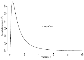
Y | η, σ² ~ INormal(η, σ²) with density function: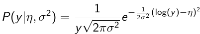

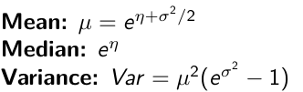
It also implies: Log( Y )~ Normal(η, σ²)

In JAGS we use: dlnorm(η, σ²)

"model {
for (i in 1:N) {
	hbf[i] ~ dlnorm(lb.0,tau.t)
}

## prior on precision parameters
tau.t ~ dgamma(1,1);

### prior on mean
lb.0 ~ dnorm(1.6,1.6);

b.0 <- exp(lb.0)

### prediction
hbf.new ~ dlnorm(lb.0,tau.t)
pred <- step(hbf.new-20)
}"

In the above example, we get the initial prior on β₀from previous data, where we derived median(b.0)=5 and V(b.0)=1/0.44=2.27
Then we take the log of the median to get η and transform the precision variable with: log(1 + V (b.0)/E (b.0)² ), then take the inverse of that to get the variance.

Parameter Interpretation

Let's consider data of the SNP rs766432 on the effect of HbF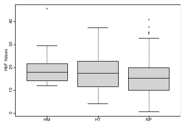

Where HT is heterzygote, HM is homozygoute and NP is common alleles.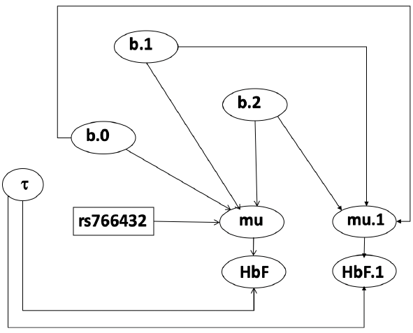

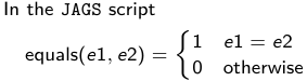
We start by creating indicators for HT and NP using the equals( , ) function in JAGS
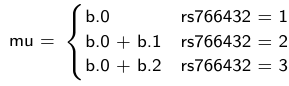
The mean of Log HbF

b.1 = the effect of HT vs HM
b.2 = the effect of NP vs HM
The hypotheses:
1. H0: b.1 = 0; HM and HT have the same effect
2. H0: b.2 = 0; HM and NP have the same effect

model.1 <- "model {
	for (i in 1:N) {
		hbf[i] ~ dlnorm(mu[i],tau.t)
		mu[i] <- b.0+b.1 *equals(rs766432[i],2)+b.2 *equals(rs766432[i],3)
	}
	## prior on precision parameters
	tau.t ~ dgamma(1,1);
	### prior on mean given precision
	b.0 ~ dnorm(0, 0.001);
	b.1 ~ dnorm(0, 0.001);
	b.2 ~ dnorm(0, 0.001);
	### prediction
	lmu.1 <- b.0;
 	hbf.1 ~ dlnorm( lmu.1,tau.t); 
    pred.1 <- step(hbf.1-20)
	lmu.2 <- b.0+b.1; 
    hbf.2 ~ dlnorm( lmu.2,tau.t); 
    pred.2 <- step(hbf.2-20)
	lmu.3 <- b.0+b.2; 
    hbf.3 ~ dlnorm( lmu.3,tau.t); 
    pred.3 <- step(hbf.3-20)
	### fitted medians by genotypes
	mu.1 <- exp(lmu.1)
	mu.2 <- exp(lmu.2)
	mu.3 <- exp(lmu.3)
	par.b[1] <- b.0;
	qpar.b[2] <- b.1;
	par.b[3] <- b.2
	par.h[1] <- hbf.1; 
    par.h[2] <- hbf.2; 
    par.h[3] <- hbf.3;
	par.m[1] <- mu.1;
	par.m[2] <- mu.2;
	par.m[3] <- mu.3
	par.p[1] <- pred.1; 
    par.p[2] <- pred.2; 
    par.p[3] <- pred.3
}"

data.1 <- source("saudi.data.2.txt")[[1]]
model_hbf <- jags.model(textConnection(model.1), data = data.1,n.adapt = 1000)
update(model_hbf, 10000)
test_hbf <- coda.samples(model_hbf, c("par.b", "par.h", "par.m","par.p"), n.iter = 10000)
summary(test_hbf)
plot(test_hbf)
autocorr.plot(test_hbf)

To analyze the convergence we can observe normality in auto-correlation plots. If we wee substantial auto-correlation (lag > X), we can repeat the the MCMC for 100,000 simulations and sample every X steps by using thin = X in coda.samples(); where X is how often order occurs in the plot.

test_hbf <- coda.samples(model_hbf, c("par.b", "par.h", "par.m","par.p"), n.iter = 1e+05, thin = 30)

Depending on which hypothesis we are testing we could also eliminate b.1 or b.2. Or in other situations reparameterizations can reduce correlation.

ANOVA Example

In this example let's consider a study of 5 different treatment groups assigned to wear shirts with differing levels of cotton (15%, 20%, 25%, 30%, and 35%) and strength was measured. We'll code these levels as dummy variables and

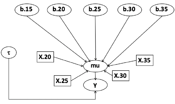
Note that since 15% is the reference group we keep it as a constant.

model.1 <- "model {
	### data model
	for(i in 1:N){
		y[i] ~dnorm(mu[i], tau)
		mu[i] <- b.15 + b.20*lev.20[i] +b.25 *lev.25[i] +
		b.30*lev.30[i] +b.35 * lev.35[i] 
    }
	###
	prior
	b.15 ~dnorm(0,0.0001); ## referent group
	b.20 ~dnorm(0,0.0001);
	b.25 ~dnorm(0,0.0001);
	b.30 ~dnorm(0,0.0001);
	b.35 ~dnorm(0,0.0001);
	tau ~dgamma(1,1)
	### difference in strength between level 3 (25%) and level 4 (30%)
	b.30.25 <- b.30-b.25
	### estimated strength in groups (30%)
	strength[1] <- b.15
	strength[2] <- strength[1]+b.20
	strength[3] <- strength[1]+b.25
	strength[4] <- strength[1]+b.30
	strength[5] <- strength[1]+b.35
}"

ANCOVA Example

These are models that include a continuous covariate and a categorical variable with 2 categories.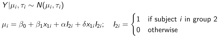

When the slope differs in the 2 groups and the lines are not parallel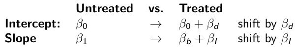

model.1 <- "model{
  ### data model
  for(i in 1:N){
      hbf_after[i] ~dlnorm(mu[i],tau)
      Lhbf_baseline[i] <- log(hbf_baseline[i])
      mu[i] <- beta.0 + beta.d*Drug[i] +
      beta.b*(Lhbf_baseline[i]-mean(Lhbf_baseline[])) +
      beta.i*Drug[i] *(Lhbf_baseline[i]-mean(Lhbf_baseline[]))
  }
  ### prior density
  beta.0 ~ dnorm(0,0.0001)
  beta.d ~dnorm(0, 0.0001)
  beta.b ~dnorm(0, 0.0001)
  beta.i ~dnorm(0,0.0001)
  tau ~ dgamma(1,1);
  ### inference
  parameter[1] <- beta.0
  parameter[2] <- beta.d
  parameter[3] <- beta.b
  parameter[4] <- beta.i
}"
### generate data
Drug = rep(0, nrow(hbf.data))
Drug[treatment == "Hy"] <- 1
table(Drug, hbf.data$Drug)
data.1 <- list(N = as.numeric(nrow(hbf.data)), hbf_baseline = hbf_baseline, hbf_after = hbf_after, Drug = Drug)
model_mean <- jags.model(textConnection(model.1), data = data.1,n.adapt = 1000)
update(model_mean, 10000)
test_mean <- coda.samples(model_mean, c("parameter"), n.iter = 10000)

So if the interaction term is significant then we would conclude the treatment has an effect

Missing Values

Treat missing values in the response as unknown parameters and JAGS will generate them as a form of imputation. Missing data in the covariates however is not so easy.

Model Selection: DIC

Model selection based on marginal likelihood is most robust but difficult to implement
Often model search over many models is based on BIC using posterior estimates of parameters
Model selection for a small number of models is based on posterior intervals

Start from the deviance: -2log(P(y | β, τ ))

Deviance information Criterion:
DIC = Dbar + pD = Dhat + 2 * pD

Dbar: -2 E(log(P(y | β, τ ))) = posterior mean of the deviance
Dhat: -2 log(P(y | β^, τ^ ) = point estimate of the deviance using the posterior means of the parameters
pD: Dbar - Dhat = Effective number of parameters

The model with the smallest DIC is estimated to be the model that would best predict a replicate dataset of the same structure as the observed.

Bayesian Linear Regression

When Mean and Variance are Unknown

Predictive Distributions

Log Normal Distributions

Parameter Interpretation

ANOVA Example

ANCOVA Example

Missing Values

Model Selection: DIC

No Comments