τ = 1 / σ2 , also called **precision** <- Be aware this will be used interchangeably with variance
The density function is: [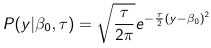](https://bookstack.mitchellhenschel.com/uploads/images/gallery/2023-02/ByOimage.png) Mean and variance: E(Y) = μ0; V(Y) = 1/τ0 + τ The Posterior Distribution for β0 is calculated using Bayes' Theorem[](https://bookstack.mitchellhenschel.com/uploads/images/gallery/2023-02/lLKimage.png) ##### When Mean and Variance are Unknown We use a Normal prior distribution for the mean β0 ∼ N(μ0, τ0) and a **Gamma** prior distribution for the precision parameter: [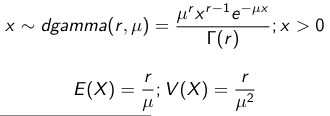](https://bookstack.mitchellhenschel.com/uploads/images/gallery/2023-02/0Drimage.png) JAGS example: ``` model.1 <- "model { for (i in 1:N) { hbf[i] ~ dnorm(b.0,tau.t) } ## prior on precision parameters tau.t ~ dgamma(1,1); ### prior on mean given precision mu.0 <- 5 tau.0 <- 0.44 b.0 ~ dnorm(mu.0, tau.0); ### prediction hbf.new ~ dnorm(b.0,tau.t) pred <- step(hbf.new-20) # hbf >= 20 }" ``` #### Predictive Distributions Given the Prior and Observed data we can compute the probability of a new observation will be greater or less than some integer threshold. The predictive distribution is a distribution of unobserved y~, that is: [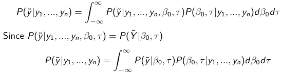](https://bookstack.mitchellhenschel.com/uploads/images/gallery/2023-02/7xDimage.png) The two sources of variability in prediction are in the parameters V(β0, τ | y) and the variability in the new observation V(y | β0, τ) - To simulate from predictive density, do repeatedly: 1. Sample one sample β0\*, τ\* from posterior β0, τ | y 2. Sample one y~ ~ N(β0\*, 1/τ\* ) - During the Gibbs sampling we generate samples values from the posterior distribution β0, τ | y - So Generating y~ ~ N(β0, τ | y) will produce the correct predictive distribution samples. P(y~ > 20 | data) is the proportion of y~ > 20 #### Log Normal Distributions Since in the example above the outcome distribution can only be positive we can use a Log-Normal distribution, a continuous distribution with support for values y > 0. [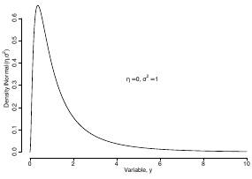](https://bookstack.mitchellhenschel.com/uploads/images/gallery/2023-02/vEWimage.png) Y | η, σ2 ~ INormal(η, σ2) with density function: [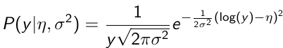](https://bookstack.mitchellhenschel.com/uploads/images/gallery/2023-02/ye6image.png) [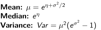](https://bookstack.mitchellhenschel.com/uploads/images/gallery/2023-02/NX5image.png) It also implies: Log( Y )~ Normal(η, σ2) In JAGS we use: dlnorm(η, σ2) ``` "model { for (i in 1:N) { hbf[i] ~ dlnorm(lb.0,tau.t) } ## prior on precision parameters tau.t ~ dgamma(1,1); ### prior on mean lb.0 ~ dnorm(1.6,1.6); b.0 <- exp(lb.0) ### prediction hbf.new ~ dlnorm(lb.0,tau.t) pred <- step(hbf.new-20) }" ``` In the above example, we get the initial prior on β0 from previous data, where we derived median(b.0)=5 and V(b.0)=1/0.44=2.27 Then we take the log of the median to get η and transform the precision variable with: log(1 + V (b.0)/E (b.0)2 ), then take the inverse of that to get the variance. #### Parameter Interpretation Let's consider data of the SNP rs766432 on the effect of HbF [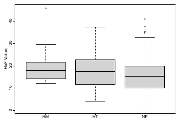](https://bookstack.mitchellhenschel.com/uploads/images/gallery/2023-02/edaimage.png) Where HT is heterzygote, HM is homozygoute and NP is common alleles. [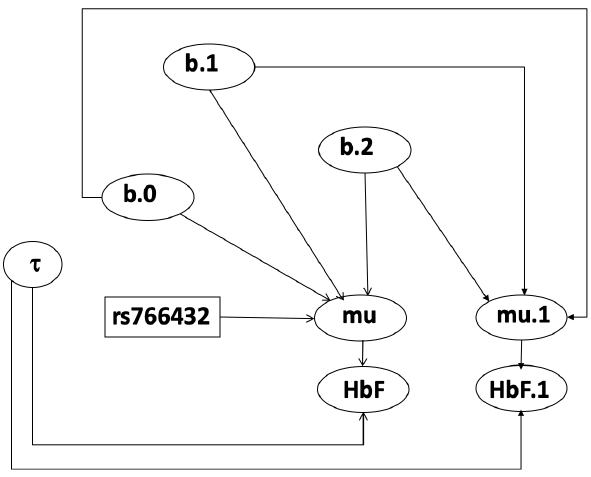](https://bookstack.mitchellhenschel.com/uploads/images/gallery/2023-02/HRIimage.png) - We start by creating indicators for HT and NP using the equals( , ) function in JAGS [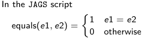](https://bookstack.mitchellhenschel.com/uploads/images/gallery/2023-02/iVLimage.png) - The mean of Log HbF [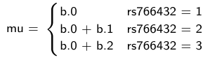](https://bookstack.mitchellhenschel.com/uploads/images/gallery/2023-02/hd7image.png) b.1 = the effect of HT vs HM b.2 = the effect of NP vs HM - The hypotheses: 1. H0: b.1 = 0; HM and HT have the same effect 2. H0: b.2 = 0; HM and NP have the same effect ``` model.1 <- "model { for (i in 1:N) { hbf[i] ~ dlnorm(mu[i],tau.t) mu[i] <- b.0+b.1 *equals(rs766432[i],2)+b.2 *equals(rs766432[i],3) } ## prior on precision parameters tau.t ~ dgamma(1,1); ### prior on mean given precision b.0 ~ dnorm(0, 0.001); b.1 ~ dnorm(0, 0.001); b.2 ~ dnorm(0, 0.001); ### prediction lmu.1 <- b.0; hbf.1 ~ dlnorm( lmu.1,tau.t); pred.1 <- step(hbf.1-20) lmu.2 <- b.0+b.1; hbf.2 ~ dlnorm( lmu.2,tau.t); pred.2 <- step(hbf.2-20) lmu.3 <- b.0+b.2; hbf.3 ~ dlnorm( lmu.3,tau.t); pred.3 <- step(hbf.3-20) ### fitted medians by genotypes mu.1 <- exp(lmu.1) mu.2 <- exp(lmu.2) mu.3 <- exp(lmu.3) par.b[1] <- b.0; qpar.b[2] <- b.1; par.b[3] <- b.2 par.h[1] <- hbf.1; par.h[2] <- hbf.2; par.h[3] <- hbf.3; par.m[1] <- mu.1; par.m[2] <- mu.2; par.m[3] <- mu.3 par.p[1] <- pred.1; par.p[2] <- pred.2; par.p[3] <- pred.3 }" data.1 <- source("saudi.data.2.txt")[[1]] model_hbf <- jags.model(textConnection(model.1), data = data.1,n.adapt = 1000) update(model_hbf, 10000) test_hbf <- coda.samples(model_hbf, c("par.b", "par.h", "par.m","par.p"), n.iter = 10000) summary(test_hbf) plot(test_hbf) autocorr.plot(test_hbf) ``` To analyze the convergence we can observe normality in auto-correlation plots. If we wee substantial auto-correlation (lag > X), we can repeat the the MCMC for 100,000 simulations and sample every X steps by using thin = X in coda.samples(); where X is how often order occurs in the plot. test\_hbf <- coda.samples(model\_hbf, c("par.b", "par.h", "par.m","par.p"), n.iter = 1e+05, thin = 30) Depending on which hypothesis we are testing we could also eliminate b.1 or b.2. Or in other situations reparameterizations can reduce correlation. #### ANOVA Example In this example let's consider a study of 5 different treatment groups assigned to wear shirts with differing levels of cotton (15%, 20%, 25%, 30%, and 35%) and strength was measured. We'll code these levels as dummy variables and [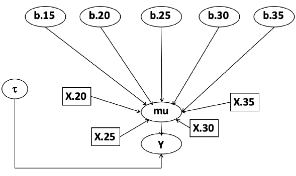](https://bookstack.mitchellhenschel.com/uploads/images/gallery/2023-02/jm7image.png) Note that since 15% is the reference group we keep it as a constant. ``` model.1 <- "model { ### data model for(i in 1:N){ y[i] ~dnorm(mu[i], tau) mu[i] <- b.15 + b.20*lev.20[i] +b.25 *lev.25[i] + b.30*lev.30[i] +b.35 * lev.35[i] } ### prior b.15 ~dnorm(0,0.0001); ## referent group b.20 ~dnorm(0,0.0001); b.25 ~dnorm(0,0.0001); b.30 ~dnorm(0,0.0001); b.35 ~dnorm(0,0.0001); tau ~dgamma(1,1) ### difference in strength between level 3 (25%) and level 4 (30%) b.30.25 <- b.30-b.25 ### estimated strength in groups (30%) strength[1] <- b.15 strength[2] <- strength[1]+b.20 strength[3] <- strength[1]+b.25 strength[4] <- strength[1]+b.30 strength[5] <- strength[1]+b.35 }" ``` #### ANCOVA Example These are models that include a continuous covariate and a categorical variable with 2 categories. [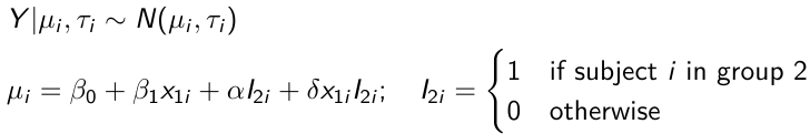](https://bookstack.mitchellhenschel.com/uploads/images/gallery/2023-02/TEWimage.png) When the slope differs in the 2 groups and the lines are not parallel [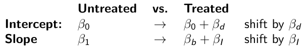](https://bookstack.mitchellhenschel.com/uploads/images/gallery/2023-02/tgYimage.png) ``` model.1 <- "model{ ### data model for(i in 1:N){ hbf_after[i] ~dlnorm(mu[i],tau) Lhbf_baseline[i] <- log(hbf_baseline[i]) mu[i] <- beta.0 + beta.d*Drug[i] + beta.b*(Lhbf_baseline[i]-mean(Lhbf_baseline[])) + beta.i*Drug[i] *(Lhbf_baseline[i]-mean(Lhbf_baseline[])) } ### prior density beta.0 ~ dnorm(0,0.0001) beta.d ~dnorm(0, 0.0001) beta.b ~dnorm(0, 0.0001) beta.i ~dnorm(0,0.0001) tau ~ dgamma(1,1); ### inference parameter[1] <- beta.0 parameter[2] <- beta.d parameter[3] <- beta.b parameter[4] <- beta.i }" ### generate data Drug = rep(0, nrow(hbf.data)) Drug[treatment == "Hy"] <- 1 table(Drug, hbf.data$Drug) data.1 <- list(N = as.numeric(nrow(hbf.data)), hbf_baseline = hbf_baseline, hbf_after = hbf_after, Drug = Drug) model_mean <- jags.model(textConnection(model.1), data = data.1,n.adapt = 1000) update(model_mean, 10000) test_mean <- coda.samples(model_mean, c("parameter"), n.iter = 10000) ``` So if the interaction term is significant then we would conclude the treatment has an effect #### Missing Values Treat missing values in the response as unknown parameters and JAGS will generate them as a form of imputation. Missing data in the covariates however is not so easy. #### Model Selection: DIC - Model selection based on marginal likelihood is most robust but difficult to implement - Often model search over many models is based on BIC using posterior estimates of parameters - Model selection for a small number of models is based on posterior intervals Start from the deviance: -2log(P(y | β, τ )) Deviance information Criterion: DIC = Dbar + pD = Dhat + 2 \* pD Dbar: -2 E(log(P(y | β, τ ))) = posterior mean of the deviance Dhat: -2 log(P(y | β^, τ^ ) = point estimate of the deviance using the posterior means of the parameters pD: Dbar - Dhat = Effective number of parameters The model with the smallest DIC is estimated to be the model that would best predict a replicate dataset of the same structure as the observed.