Introduction to Bayesian Modeling
In the frequentist approach, estimated probabilities are viewed as one of an infinite sequence of possible data of the same experiment, while Bayesian analysis is based on expressing uncertainty about unknown quantities as formal probability distributions.
Bayes Problem: Given the number of times in which an unknown event has happened and failed - Requires the chance that the probability of its happening in a single trial lies somewhere between any two degrees of probability that can be named.
Bayesian statistics used probability as the only way to describe uncertainty in both data and parameter. Everything that is not known for certain are modeled with distributions and treated as random variables. Bayesian inference focuses on the uncertainty in value of parameter and decisions which is conditional on sample data.
| Exposed |
Unexposed |
||
| Diseased |
a |
b |
m1 |
| Not Diseased |
c |
d |
m0 |
| n1 |
n0 |
n |
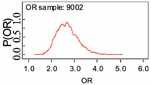
Recall the odds ratio (OR) is the probability of having an outcome (disease) compared to the probability of not having the outcome: ad / bc
Bayesian Statistics takes the point of view that OR and RR are uncertain unobservable quantities, which we can model with a probability distribution.
Prior probability: Model/probability distribution using existing data/knowledge
Posterior probability: Updated model with new and prior data; These are used in inference
Bayes theorem allows us to learn from experience and turn a prior distribution into a posterior distribution.
Bayes Theorem
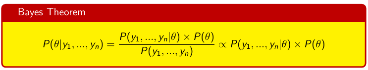
The denominator in Bayes Theorem is a normalizing constant. If a conjugate of the family of distribution then the normalizing constant can be derived.
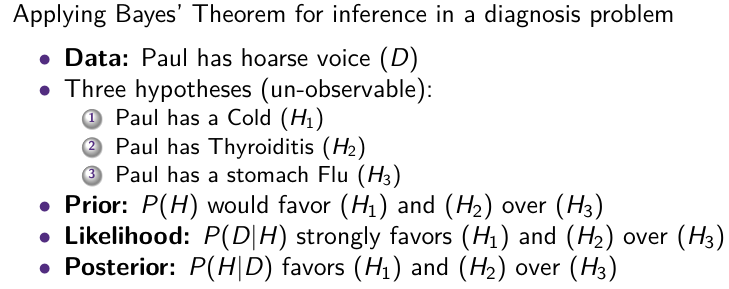
P(H) = Probability of H (Prior Density)
P(H | data) =( P(data | H)*P(H) ) / P(Data) = Posterior probability of H
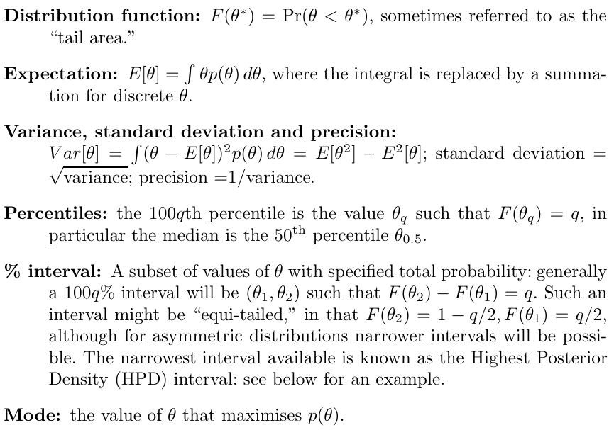
Consider a generic probability distribution p(𝜃) for a single parameter 𝜃. The probability distributions are defined as:
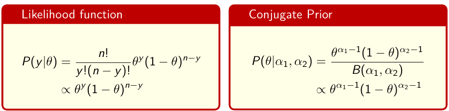
Conjugate Analysis: Beta-Binomial
In conjugate analysis the prior density for theta has the same functional form as the likelihood function.
Credible Interval
A Confidence Interval represents uncertainty we have about the method used in generating an interval that captures the true value in repeated sampling. The parameter is fixed and the interval is random.
A Credible Interval is a statement about the probability that a parameter lies in a fixed interval. The uncertainty is related to the value of the true parameter and the interval is fixed.
Markov Chain Monte Carlo (MCMC) Simulation
There are several ways to calculate the properties of probability distributions for unknown parameters. We will be focusing on using simulation of the known random variables and estimate the property of interest.
Note that there are entire classes on algorithms used for simulation, we will not go into great depth on the underlying theory.
Monte Carlo algorithms are a broad class of computational algorithms that rely on repeated random sampling to obtain numerical results.
Suppose we have a random variable X which has a probability distribution p(x) and we have an algorithm for generating a large number of independent trials x(1), x(2), ... x(T) . Then:
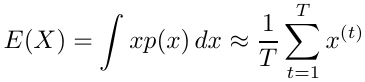
By the law of large numbers the approximation becomes exact as T approaches infinity.
Additionally, if I(l < X < u) is an indicator function where the value is 1 when X lies between l and u and 0 otherwise, the probability can be estimated with Monte Carlo integration by taking the sample average for each realization x(t)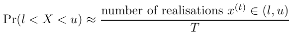
Note that, in general, MCMC methods generate a dependent sample from the joint posterior of interest, since each realisation depends directly on its predecessor.
In R:
# Step 1: Generate samples
x <- rbinom(1000, 8, 0.5)
# Represent histogram
hist(x, main = "")
# Step 2: Estimate P(X<=2) as
# Proportion of samples <= 2
sum(x <= 2)/1000
## 0.142
Gibbs Sampling
Gibbs Sampling is MCMC algorithm that reduces high dimensional simulation to lower dimensional simulations. Used in BUGS (Bayesian Inference Using Gibbs Sampling) and JAGS as the core algorithm for sampling from posterior distributions.
The algorithm generates a multi-dimensional Markov chain by splitting the vector of random variables θ into subvectors (often scalars) and sampling each subvector in turn, conditional on the most recent values of all other elements of θ. I will not go into great detail on the process because the computer does this for us.
With Gibbs sampling we can give a value to P(𝜃 > .2) or P(Y > 5), but not P(Y > 5 | 𝜃 = .2)
JAGS
JAGS is functionally for the MCMC. It is not a procedural language like R; it can be called from R. You can write complex model code in any order using a very limited syntax
The below code does the same thing as the previous R snippet but using JAGS:
library(rjags)
### model is defined as a string
model11.bug <- "model {
Y ~ dbin(0.5, 8)
P2 <- step(2 - Y)
}"
writeLines(model11.bug, "model11.txt")
# Now run the Gibbs sampling for 1000 iterations
### (Step 1) Compile BUGS model
M11 <- jags.model("model11.txt", n.chains = 1, n.adapt = 1000)
### (Step 2) Generate 1000 samples and discard
mcmc_11 <- update(M11, n.iter = 1000)
### (Step 3) Generate 10000 samples and retain for
### inference
test_11 <- coda.samples(M11, variable.names = c("P2", "Y"), n.iter = 10000)
JAGS uses directed graphical models for internal representation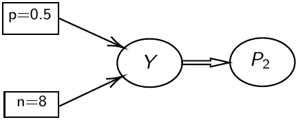
- Nodes represent variables
- Directed arrows represent conditional probability distributions
- Double arrows are mathematical functions
The joint probability distribution can be derived using Markov properties of marginal and conditional independence (next section).
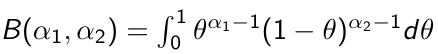
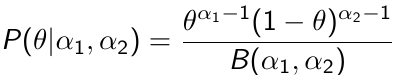
Beta Distribution
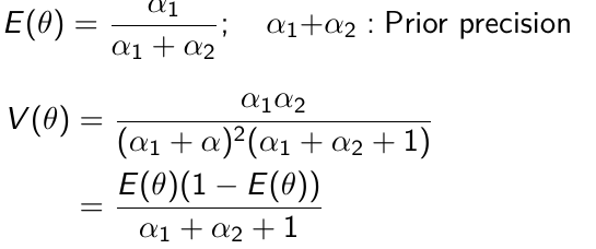
Beta is a family of probability distributions with support between 0 and 1, it is the typical choice for working with probability parameters. The density function depends on two hyper-parameters 𝛼1 and 𝛼2.
𝛼1 + 𝛼2 = effective sample size with 𝛼1 events (more on this in a later section)
Functions rbeta(), dbeta(), qbeta(), pbeta() available in R for working with Beta distributions. It's also implemented in JAGS as function dbeta( , )
The prior hyper-parameters determine the expected Y events. The posterior mean thus be written as: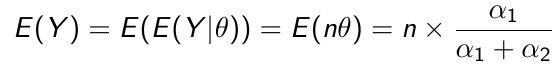
No Comments