Bayesian Logistic Regression

Let Y be an indicator for presence of disease ->    Y | p ~ Bin(p, 1)

Logistic regression models the log-ODDS (also called logit) of the mean outcome using a linear predictor.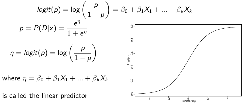

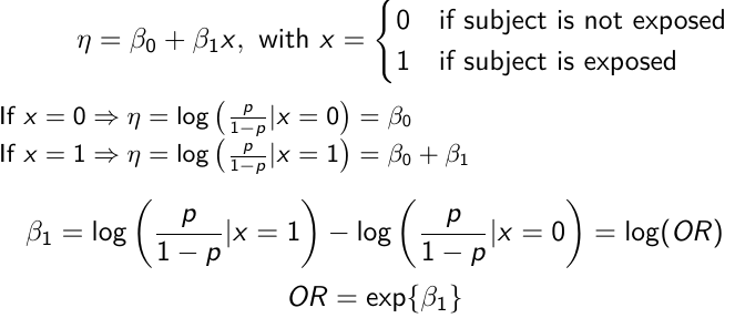
In a case-control study beta_0 is not interpretable. But the estimate of log(OR) can be interpreted correctly, given the symmetry of roles of disease/exposure

H₀: OR = 1; Log(OR) = 0; No association
H₁: OR != 1; Log(OR) != 0; Significant association

The Frequentist approach to test the above is to fit a logistic regression in R using the function glm() and assess the OR.

In Bayesian formulation we need to identify the parameters in our prior model, and the parameters we wish to estimate to form a posterior distribution to assess the OR. We can compute the probability that OR > 1, < 1 or != 1 using a small range.

Ex. Below we model 2 parameters, beta_0 and beta_1, in a DAG model: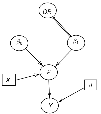

Because there's no constraint on the beta regression parameters, it is common to assume a normal distribution.
The magnitude of variance reflects the amount of uncertainty

In the below code:

• We loop to specify each observation
• Y.D[i] =
  • 1 if subject i has the disease
  • 0 if subject i does not have the disease
• X.E[i] =
  • 1 if subject i has been exposed
  • 0 if subject i has not been exposed

# Analysis with JAGS
library(rjags)

model.1 <- "model{
### data model
for(i in 1:N){
    Y.D[i] ~ dbin(p[i], 1)
    logit(p[i]) <- beta_0 + beta_1*X.E[i]
}
OR <- exp(beta_1)
pos.prob <- step(beta_1)
### prior
beta_1 ~ dnorm(0,0.0001)
beta_0 ~ dnorm(0,0.0001)
 0 i th subject unexposed
}"
# In R Data stored as a list
data.1 <- list(N = 331, X.E = X.E, Y.D = Y.D)
# Compile model (data is part of it!); `adapt` for 2,000 samples
model_odds <- jags.model(textConnection(model.1), data = data.1,
n.adapt = 2000)
update(model_odds, n.iter = 5000) # 5,000 burn-in samples
# Get 10,000 samples from the posterior distribution of OR, beta_0,beta_1
test_odds <- coda.samples(model_odds, c("OR", "beta_1", "beta_0"), n.iter = 10000)
plot(test_odds)
summary(test_odds)

In the output, we'll often look for the point estimate to be the posterior mean. However, when posterior density is skewed, posterior median is sometimes preferable.

Asymptotic Approximation

When the sample size is large enough, one can use an asymptotic approximation of the posterior distribution of the parameters.

When the sampling distribution is a member of the exponential family (Normal, Binomial, Poisson, or Gamma), then the posterior distribution of the parameters is (approximately) normally distribution: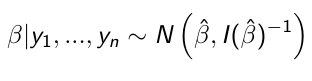
[1]
beta_hat is the ML (maximum likelihood) estimate of beta
I(beta_hat)^-1 is the Fisher Information matrix, evaluated in the ML estimate of beta

Based on the Maximum likelihood theory, asymptotically:
[2]

We don't need a prior in [1] because we have a lot of data. Results in [1] and [2] are close because the prior is weighted low because of the high sample size.

Gibbs Sampling for Logistic Regression

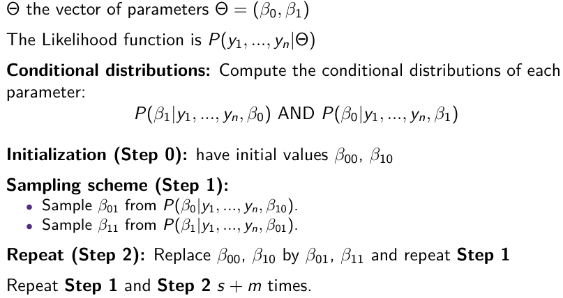
Posterior Inference

Obtain s + m sample for each parameter
Throw away the first s values (burn-in)
Use the m samples with Monte Carlo algorithms to carry out inference:

1. Point Estimates - Posterior means or medians
   

   

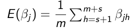
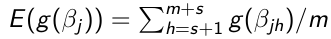
2. Transformations - Any function of the parameters
   

   

3. Posterior Density - Density estimation methods to estimate the posterior density of parameters
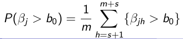
4. Tail probabilities
   

   

Marginal and Conditional Independence

Two random variables, X and Y, are independent (denoted by X ⊥ Y) if an only if:
P(X, Y) = P(X)P(Y); Joint p.m.f. for joint density = Marginal p.m.f. or marginal density

Given three random variables, X, Y and X, are conditionally independent given Z (denoted by Y  ⊥  Y | Z) if and only if:
P(X, Y | Z) = P(X | Z) P(Y | Z)

There is no relation between marginal and conditional independence (Simpson Paradox)

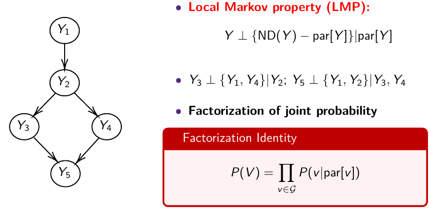
The directed graph specifies conditional and marginal independence through two properties; The Local Markov Property (LMP) specifies that we need to specify only the distribution of nodes given their parents. The Global Markov Property (GMP) is used internally to derive the conditional distributions of each node given all others.

Local Markov Property (LMP)

Descendants of Y [D(Y)] are all nodes reached from Y with a directed path
Non-descendants of Y [NS(Y)] - all nodes minus the descendant nodes

Global Markov Property (GMP)

The node is independent of everything else in the network given its Markov Blanket.

For each node, list the Markov blanket: Markov blanket of A: the parents of A, the children of A and the parents of the children of A

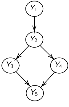
Y_1 independent of Y_3, Y_4, Y_5, given Y_2
MB(Y_1) = { Y_2 }; MB(Y_2) = { Y_1, Y_3, Y_4 }

The LMP is used to specify the priors and the likelihood
The GMP is used to generate the conditional distributions to run the Gibbs Sampling

Bayesian Hypothesis Testing: Prior Odds

On each hypothesis we  have a prior probability:
P(H₀) = P(M₀) and P(H_a) = P(M₁)

Use the data to compute the posterior probability of each hypothesis: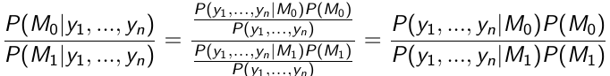

This equates to:
Posterior ODDs = Bayes Factor * Prior Odds
We accept the hypothesis with maximum posterior probability (0 - 1 loss)

The Bayes Factor is the ratio of the likelihood functions computed for models M0 and M1

If P(M0) = P(M1) then the posterior probability of M1 is larger than the posterior probability of M0

We can also assign weights to adjust the probability of making errors: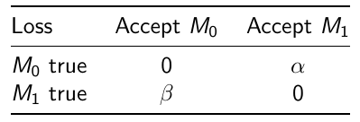

Where alpha would be the loss incurred if M1 is accepted when M0 is true
and beta is  the loss incurred if M0 is accepted when M1 is true.