Mutlivariate and Joint Models for Longitudinal Data

Longitudinal studies are commonly designed in many research fields in order to see changes over a time interval shared by all participants. Joint modeling consists of two interlinked sub-models with any type of outcome (continuous, binomial, etc). One of the most commonly used is longitudinal sub-model is the linear mixed effect model and a cox proportional hazard with time-to-event sub-model.

Joint modeling reduces the bias of parameter estimates by accounting for the association between the longitudinal and time-to-event data. In clinical trials this often leads to more efficient estimation of the treatment effect on both sub-model outcomes.

Let's assume Y_i1and Y_i2 are two outcomes measured on subject i. We can attempt to specify a joint density f(y_i1, y_i2), but this is only feasible if we assume certain things about the marginal association among the longitudinally measured elements within each of the outcome vectors. This is easier when both outcomes and conditional models are of the same type, but this is not a requirement. When Y_i1and Y_i2 are of different types, or in the case of unbalanced data, this becomes cumbersome. Thus, extensions to higher dimensional data involves considerable challenges as this would require assumption on larger covariance structure and higher order associations.

Conditional Models

We can avoid direct specification of the joint density f(y_i1, y_i2) are and reduce the modeling tasks by specifying a model for each outcome separately:
f(y_i1, y_i2) = f(y_i1| y_i2) f(y_i2)
= f(y_i2| y_i1) f(y_i1)

The main drawback is that this requires reflection about the plausible association between Y_i1and Y_i2 that may be inappropriate in some settings. For example, in a clinical trial with two main post-randomization outcomes conditioning on one of the outcomes may attenuate (make smaller) the treatment effect on the other. Also, it is difficult to implement in high-dimension data.

Shared-Parameter Models

In previous chapters we've seen how random effects can be used to generate an association structure between repeated measurements of a specific outcome. We can use a similar approach to generate association between two outcomes.

\( f(y_{i1}, y_{i2}) = \int f(y_{i1}, y_{i2} | b) f(b) db = \int f(y_{i1} | b) f( y_{i2} | b) f(b) db \)

Where b is a vector of ranom effects common to the outputs Y_i1and Y_i2, and assume independence of both outcomes conditional on b.

Again the outcomes do not have to be of the same type, but we assume b represents a common set of unobserved characteristics of the subject that governs both models.

Examples:

Let Y_i1represent a vector of longitudinal continuous outcomes and Y_i2= (U_i, 𝛿_i) with U = min(T_i, C_i) with T_i as the potential time to the event of interest, C_i as the potential censoring time, and 𝛿_i = I(T_i <= C_i). Let Y_i1follow a random intercept model:
Y = β₀ + b_0i + β₁t + ε_i1t
and let the event time of interest follow a proportional hazard model so that: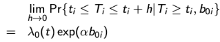

where λ₀(t) is an unspecified baseline hazard function

In another case, the shared-parameter random effect models may imply very strong assumptions for the association structure between outcomes. Consider this example where Y_i1and Y_i2 are two longitudinal continuous outcomes that share a common random intercept: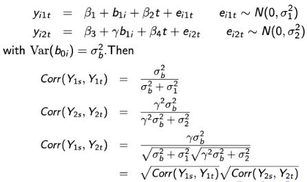

The joint random-effects imply more flexible correlation patterns. Consider this example where Y_i1and Y_i2 are dependent on separate random effects b1 and b2 which are themselves correlated: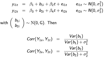

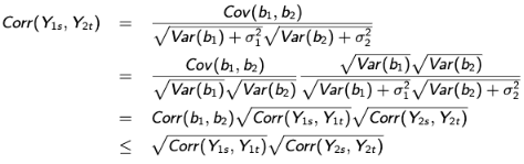
This demonstrates the role of the correlation between the outcome-specific random effects in the between-process outcome correlation at any two time points. The restriction is imposed by the shared-parameter model is relaxed in the same sense that the model no longer assumes the product of within process correlations equals the between-process correlation and thus allows a more general dependence structure.

In many situations (especially when we have multiple outcomes/high-dimensional data) the previous methods will not be feasible to estimate. Methods that reduce the dimensions are more appropriate. The idea is to use a factor-analytic or principal component type of analysis to reduce the dimensions. After, the estimated factors can be analyzed using any of the classical longitudinal models. The disadvantage is that the inferences are restricted to the factors and cannot be extended to the original outcome variables, so certain assumptions need to be imposed in the case of unequally spaced observations or unbalanced designs.

Defining the Generalized Linear Models

For a bi-variate response Y_i = (Y_i1, Y_i2)', we can assume a general model in the form of: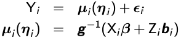

with g^-1 as the inverse link function which is allowed to change for each univariate outcome and b_i ~ N(0, G).

A general first-order approximate expression for the variance-covariance matrix of Y_i is:
Var(Y_i) ~= Δ_i Z_i GZ'_iΔ'_i + V_iWhere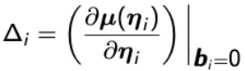
and
and R( α ) is the correlation matrix and the Ξ_i is a diagonal matrix with over-dispersion parameters along the diagonal: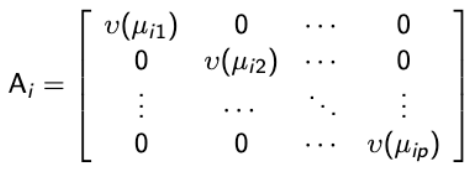

If there are no random effects then the model is referred to as a marginal generalized linear model (MGLM). For the special case of a continuous and binary endpoint the MGLM is in the form of: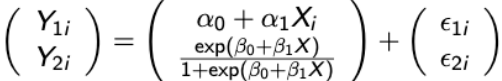

with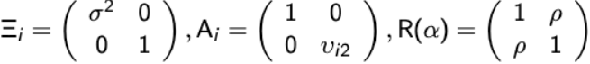

v_i2 = μ_i2(1-μ_i2)

In a shared parameter the variance of Y_i is approximately equal to: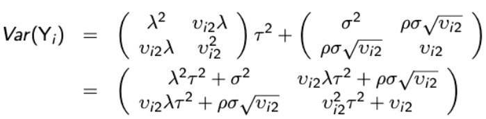
As a result the approximate correlation among the two outcomes is: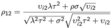

The correlation depends on the fixed effects through v_i2

SAS Code

libname s857 "/Datasets";
options fmtsearch=(s857.formats);
options nofmterr;

proc mixed data=s857.Tbi;
class sex naccid  status;
model Mem1=time  naccageb status sex time*educ time*naccageb  /solution;
random Int time/sub=naccid;
run;

proc mixed data=s857.Tbi;
class sex naccid  status;
model Att1=time  naccageb status sex time*educ time*naccageb  /solution;
random Int time/sub=naccid;
run;

/* Multivariate models  */
data s857.tbi_long;
length scale $10;
set s857.tbi;
Outcome=Mem1;scale='Memory';output;
Outcome=Att1;scale='Attention';output;
keep Outcome Scale time trauma_dich dep2yrs status sex educ naccageb naccid;
run;
proc mixed data=s857.tbi_long covtest method=ML;
class Scale sex naccid  status;
model Outcome=Scale*time Scale*naccageb Scale*status Scale*time*status
 Scale*sex Scale*time*educ Scale*time*naccageb  /solution;
random Int time/sub=naccid;
*random int/sub=Scale type=un;
run;

proc nlmixed data=s857.tbi_long;
parms b0=-0.17 b1=0.43 b2=0.39 b3=-0.83 b4=0.08 b5=-0.01
s2e_mem=0.361 g11=0.60
	c0=0.05 c1=-0.05 c2=0.5 c3=0.1 
s2e_att=0.19;
if Scale='Memory' then do;
	mean=b0+b1*time + b2*status + b3*sex +b4*time*status +b5*time*naccageb  +u1 ;
	ll = -0.5*log(3.14159265358) - log(sqrt(s2e_mem)) -0.5*(outcome-mean)**2/(s2e_mem);
end;
if Scale='Attention' then do;
	mean=c0+c1*time + c2*status + c3*time*status  +u1;
	ll = -0.5*log(3.14159265358) - log(sqrt(s2e_att)) -0.5*(outcome-mean)**2/(s2e_att);
end;
model outcome~general(ll);
random  u1~normal([0],[g11]) subject=naccid;
run;

/*Shared parameter model*/
title 'Memory';
proc mixed data=s857.tbi covtest method=ML;
class trauma_dich sex naccid  status;
model Mem1=time status  sex time*status time*naccageb  /solution;
random intercept/sub=naccid;
run;
title 'Attention';
proc mixed data=s857.tbi covtest method=ML;
class trauma_dich sex naccid  status;
model Att1=time /solution;
random intercept/sub=naccid;
run;

proc nlmixed data=s857.tbi_long;
parms b0=-0.13 b1=0.43 b2=0.39 b3=-0.83 b4=0.08 b5=-0.01
s2e_mem=0.361 g11=0.60
	c0=0.05 c1=-0.05 c2=0.5 c3=0.1 gamma=0.20
s2e_att=0.19;
if Scale='Memory' then do;
	mean=b0+b1*time + b2*status + b3*sex +b4*time*status +b5*time*naccageb  +u1 ;
	ll = -0.5*log(3.14159265358) - log(sqrt(s2e_mem)) -0.5*(outcome-mean)**2/(s2e_mem);
end;
if Scale='Attention' then do;
	mean=c0+c1*time + c2*status + c3*time*status  +gamma*u1;
	ll = -0.5*log(3.14159265358) - log(sqrt(s2e_att)) -0.5*(outcome-mean)**2/(s2e_att);
end;
model outcome~general(ll);
random  u1~normal([0],[g11]) subject=naccid;
run;
proc nlmixed data=s857.tbi_long;
parms b0=-0.13 b1=0.43 b2=0.39 b3=-0.83 b4=0.08 b5=-0.01
s2e_mem=0.361 g11=0.60 g22=.01
	c0=0.05 c1=-0.05  c2=-0.3 c3=-0.1 gamma=1 g33=0.01
s2e_att=0.19;
if Scale='Memory' then do;
	mean=b0+b1*time + b2*status + b3*sex +b4*time*status +b5*time*naccageb  +u1 +u2*time;
	ll = -0.5*log(3.14159265358) - log(sqrt(s2e_mem)) -0.5*(outcome-mean)**2/(s2e_mem);
end;
if Scale='Attention' then do;
	mean=c0+c1*time + c2*status + c3*time*status  +gamma*u1 +u3*time;
	ll = -0.5*log(3.14159265358) - log(sqrt(s2e_att)) -0.5*(outcome-mean)**2/(s2e_att);
end;
model outcome~general(ll);
random  u1 u2 u3~normal([0,0,0],[g11,0,g22,0,0,g33]) subject=naccid;
run;
proc nlmixed data=s857.tbi_long;
parms b0=-0.13 b1=0.43 b2=0.39 b3=-0.83 b4=0.08 b5=-0.01
s2e_mem=0.361 g11=0.60 g22=.01 g12=0.01
	c0=0.05 c1=-0.05  c2=-0.3 c3=-0.1  
s2e_att=0.19;
if Scale='Memory' then do;
	mean=b0+b1*time + b2*status + b3*sex +b4*time*status +b5*time*naccageb  +u1 ;
	dens = -0.5*log(3.14159265358) - log(sqrt(s2e_mem)) -0.5*(outcome-mean)**2/(s2e_mem);
	ll=dens;
end;
if Scale='Attention' then do;
	mean=c0+c1*time + c2*status + c3*time*status  +u2;
	dens = -0.5*log(3.14159265358) - log(sqrt(s2e_att)) -0.5*(outcome-mean)**2/(s2e_att);
	ll=dens;
end;
model outcome~general(ll);
random  u1 u2~normal([0,0],[g11,g12,g22]) subject=naccid;
run;

/*
if dist='Binary' then do;
		eta=v0 + v1*u1   ;
		p=exp(eta)/(1+exp(eta));
		ll = (outcome)*log(p) + (1-outcome)*log(1-p);
end;
*/

Mutlivariate and Joint Models for Longitudinal Data

Conditional Models

Shared-Parameter Models

Defining the Generalized Linear Models

SAS Code

No Comments