Multi-Level Modeling

Recall the core of mixed models is that they incorporate fixed and random effects. While single  level models assume one variance, subjects within the same level are correlated in terms of σ0j2 + σ1j2Xij + εij

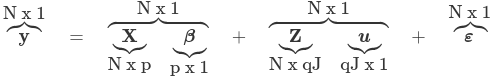
Where y is an N*1 column vector of the outcome
X is a N*p matrix of the p predictors
β is a p*1 matrix of the fixed effects regression coefficents
Z is the N*qJ design matrix for the random effects and J clusters and q random effects
u is a qJ*q vector of q random effects for J clusters/high-level units

Two Level Multi-Level Modeling

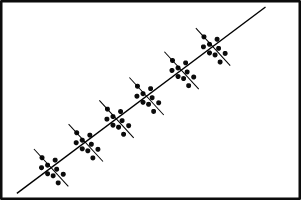
MLM is designed to account for hierarchical or clustered structured data. It is especially useful when the "assumption of independence" is violated. Ex. patients by the same doctor, since patients with the same doctor might be more similar.

Using MLMs we can account for repeated measures nested within the individual unit of analysis, as well as comparing units in one 'cluster' to another.

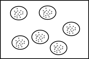
There are multiple ways to deal with hierarchical data. A simple approach is to aggregate, for example if 10 patients are sampled from each doctor we could take the average of all patients within a doctor rather than using individual patients' data. This would lead to consistent effect estimates and standard errors, but it does not really take advantage of all the data so we lose power.

Another approach is to analyze data from one high-level unit at a time, coming up with a regression model for every cluster. But again this does not make full use of the data.

The individual regressions have many estimates and lots of data but is noisy, and the aggregate method is less noisy but loses important differences by averaging all samples within each doctor. Linear mixed models (also called multi-level models) can be thought of as a trade off between these two alternatives.

Random Effects

Random effects capture cluster variability, but they can only exist for a lower level variable. There must be at least one random effect for it to be a multilevel model (but not all random effects have to be included). Typically the intercept is random, which can be thought of as everyone having a slightly different mean adjusted for no other factors. Models with overly complicated random effects may not converge.

As for choosing the structure of the random effects, the most common are unstructured (un) and variance components (VC, this is the default in SAS). So usually the best practice is to try different structures and observe the model fit, but sometimes specifying this structure is not necessary.

Three Level Multi-Level Models

An example of three level data might be schools/classrooms/students. Everything that applies to 2-level models applies to 3-level models as well. These models can have random effects for the 2nd and 3rd level, and must be either completely interdependent or non-interdependent; this requires analysis.

SAS Code

Below is sample SAS code for a campus survey with random effects for ID and campus; In this case the data is nested both within the individual and the campus:

proc mixed data=Final covtest;
class Fake_ID Fake_Campus
(ref="Atlanta") App_Status Discipline
(ref="Engineering/Computer Sciences") ;
model RUCAGRXPRSPOLI = Fake_Campus
Svy_Yr|App_Status svy_YR|Fake_Campus /solution ;
random intercept / type=vc sub=Fake_ID;
random intercept / type=vc sub=Fake_Campus;
run;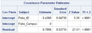

The intercept is the estimate between-subject variance
The residual is the estimated within-subject variance
Effects are significant which means it is okay to include random effects in the model

*2 Level Proc Mixed;
PROC MIXED data=data COVTEST;
CLASS ID;
MODEL DV = Predictor1/CL S DDFM=satterth;
RANDOM INTERCEPT Predictor1 / SUB=ID TYPE=UN;
RUN;

*3 Level Proc Mixed;
PROC MIXED data=data COVTEST;
CLASS DAY ID;
MODEL DV = Predictor1/CL S DDFM=satterth;
RANDOM INTERCEPT Predictor1 / SUB=DAY(ID) TYPE=UN;
RANDOM INTERCEPT Predictor1 / SUB=ID TYPE=UN;
RUN;