Linear Mixed Effects Models I

Here we'll be considering an alternative approach for analyzing longitudinal data using linear mixed effects models. These models have some subset of the individual parameters vary randomly from one subject to another, thereby accounting for sources of natural heterogeneity in the population.

Fixed effects are the population characteristics that are assumed to be shared by all subjects
Random effects are characteristics, unique for each subject
The combination of both gives rise to mixed effect models

We can write the linear mixed effects model as:
Y_i = X_i β + Z_ib_i + e_i
Where:

β is a s*1 vector of fixed effects
b_i is a q*1 vector of random effects (which follows ~N(0, G) we will see below)
e_i is an n_i*1 vector of within subject errors (~N(0, R_i)),
X_i is an n_i*s matrix of covariates,
Z_i is a n_i*q matrix of covariates with q <= s

We usually assume R_i = σ²I_n, where I_n is an n_i*n_i identity matrix with b_i and e_i mutually independent.

Model Formulation

The simplest mixed effects model for longitudinal data is:

Where b_i (some random intercept) and e_ij (error) are independent.

The marginal mean response in the population is: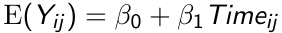

The response for the i^th subject at the j^th measurement occasion differs from the population mean response by a subject effect b_i, and a within subject measurement error e_ij.

The conditional mean response for any individual:

The residuals of profile analysis and parametric curves (ϵ_ij) and parametric curves such that ϵ_ij= b_i + e_ij

Variance and Covariance Structure

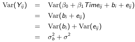
Similarly, the marginal covariance between any pair of responses: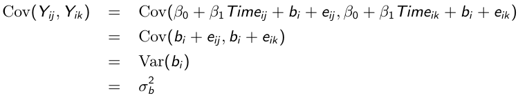

With some linear algebra we can write the variance-covariance matrix as follows: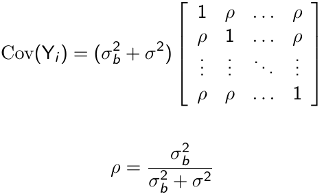

Where ρ is called the intra-cluster correlation coefficient. For ρ > 0, the random intercept mixed effects model is observationally equivalent to a compound symmetry model.

Random Intercept and Slope Model

As the name suggests, this adds a random effect for both the slope and intercept.

Consider the following model:

Where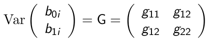

So the variance of each response varies with the time it was taken: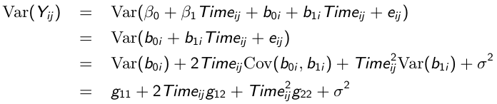

And likewise the covariance between any pair of responses: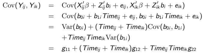

Comparing Mixed Effects Models

Inference with respect to random and fixed effects can be carried out using methods described in the previous lecture for the marginal models. For the nested models, a LR test with REML may be used (which follows a chi-squared dist with 2 degrees of freedom) while non-nested models use AIC or BIC.

Empirical BLUP

In some cases we are interested in subject-specific rather than population-averaged predictions. Mixed effect models are appropriate for this analysis. The empirical best linear unbiased predictor (BLUP) of b_i conditional on the observed vector of responses Y_i is given by:

Given the empirical BLUP, b^_i the i^th subject's predicted mean is: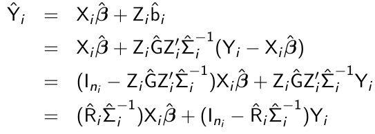

The empirical BLUP is a weighted average of the population-averaged mean X_ibeta_hat and the observed response of the i^th subject, Y_i
The empirical BLUP shrinks the i^th subject's predicted mean towards the population-averaged mean
The amount of shrinkage depends on teh relative magntude of the within-subject variability R_i relative to the sum from i, varying weight is assigned to the population-averaged mean X_ibeta_hat

Conclusion

Unlike the models we have seen up to now, mixed effects models explicitly distinguish between-subject and within-subject sources of variability.
The induced covariance structure is very parsimonious, with only a few number of parameters
They can be used to predict subject-specific mean response trajectories over time
They are very flexible in accommodating any kind of imbalance in the data, including the number and timing of measurement occasions.

SAS Code

/************************************************
* Six cities study of air pollution and health	*
*************************************************/
data fev1;
set s857.fev1;
lgfevht=Log_FEV1_-logHgt;
t=age;
run;
proc sgplot data=fev1  noautolegend ;
	* spaghetti plot;
	yaxis min = -0.3 max = 1;
	reg x=age y=lgfevht 
    / group = id nomarkers LINEATTRS = (COLOR= gray PATTERN = 1 THICKNESS = 1) ;
	* overall spline;
	reg x=age y=lgfevht 
    / nomarkers LINEATTRS = (COLOR= red PATTERN = 1 THICKNESS = 3) ;
run;
quit;
proc mixed data=fev1 covtest;
class t;
model Log_FEV1_=age logHgt Init_Age logInitHgt/s chisq;
repeated  t/type=cs subject=id R Rcorr;
run;
proc mixed data=fev1 covtest method=REML;
model Log_FEV1_=age logHgt Init_Age logInitHgt/s chisq ;
random intercept /type=un subject=id G V;
run;
proc mixed data=fev1 covtest method=REML;
model Log_FEV1_=age logHgt Init_Age logInitHgt/s chisq;
random intercept age/type=un subject=id G V;
run;

proc mixed data=fev1 covtest;
model Log_FEV1_=age logHgt Init_Age logInitHgt/s chisq;
random intercept logHgt/type=un subject=id G V;
run;


proc mixed data=fev1 covtest method=REML;
model Log_FEV1_=age logHgt Init_Age logInitHgt/s chisq;
random  intercept age logHgt/type=un subject=id G V;
run;

/************************************************
* Study of influence of menarche on changes in body fat *
*************************************************/

proc sgplot data=s857.fat  noautolegend ;
	* spaghetti plot;
	yaxis min = 0 max = 50;
	reg x=time_men y=Perc_BF 
    / group = id nomarkers LINEATTRS = (COLOR= gray PATTERN = 1 THICKNESS = 1) ;
	* overall spline;
	reg x=time_men y=Perc_BF
    / nomarkers LINEATTRS = (COLOR= red PATTERN = 1 THICKNESS = 3) ;
run;
quit;

   ods graphics on; 

   proc loess data=s857.fat plots=all;
      model Perc_BF = time_men;
   run;
 ods graphics off;

 data fat;
 set s857.fat;
 knot=max(time_men,0);
 run;
ods output solutionr=bluptable;
*ods trace on;
*ods listing;
 proc mixed data=fat covtest;
 model Perc_BF = time_men knot/s chisq outpred=yhat outpm = pred1f;
 random intercept time_men knot/type=un subject=id G V solution;
run;
*ods trace off;
ods close;

data yhat;
set yhat;
rename Pred=Pred_r;
run;
data Prediction;
merge yhat pred1f;
keep id pred pred_r time_men perc_BF;
run;

data prediction_long;
length Scale $20;
set prediction;
y=pred;Scale="Average prediction";output;
y=pred_r;Scale="Subject prediction";output;
y=perc_bf;Scale="Raw Data";output;
run;
goptions reset=all;
symbol1 c=blue  v=star   h=.8 i=j      w=5;
symbol2 c=red   v=dot    h=.8 i=j      w=1;
symbol3 c=green   v=squarefilled    h=.8 i=j      w=1;
axis1 order=(0 to 50 by 10) label=( 'Predicted % Body Fat');

proc gplot data=Prediction_long;
where id=10;
plot y*time_men=Scale/ vaxis=axis1 ;
run;
quit;

/************************************************
* Repeated CD4 counts data from AIDS clinical trial.*
*************************************************/
data CD4;
set s857.CD4;
knot=max(week-16,0);
if trt=. then treatment=.;
else if trt<4 then treatment=1;
else treatment=2;
run;
 ods graphics on; 

proc transreg ss2 data=cd4;
      model identity(log_cd4) = class(treatment / zero=none) *
                          smooth(week / sm=80);
      output p;
   run;
  
 ods graphics off;
proc mixed data=cd4 covtest;
class treatment;
model log_cd4=week knot treatment*week treatment*knot/s chisq;
random intercept  week knot/type=un subject=id G V;
run;

proc mixed data=cd4 covtest;
class treatment;
model log_cd4= week knot treatment*week treatment*knot/s chisq;
random intercept  week knot/type=un subject=id G V;
contrast'Interaction test' treatment*week 1 -1, 
							treatment*knot 1 -1;
contrast 'Slope test' treatment*week 1 -1  treatment*knot 1 -1;
run;

proc mixed data=cd4 covtest;
class treatment;
model log_cd4=week knot treatment*week treatment*knot Age Gender/s chisq outpred=random;
random intercept  week knot/type=un subject=id G V solution;
ods output solutionr=sr(keep=effect subject estimate probt);
run;
proc print data=sr;
where effect='Week' and Estimate<0 and probt<0.05;
run;