Generalized Linear Mixed Effects Models

Generalized Linear Mixed Models (GLMMs) are an extension of linear mixed models to allow response variables from different distributions (such as binary or multi-nomial responses). Think of it as an extension of generalized linear models (e.g. logistic regression) to include both fixed and random effects.

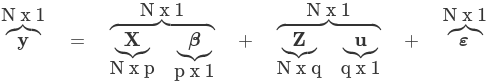
• The general form of the model is:      y_ij = X_ij β + Z_ij b_i + ε
  • y (or sometimes η) is a N*1 column vector of the dependent (outcome) variable
    
  • X is a N*p of the p predictor variables
  • Z is the N*q design matrix for q random effects (the random complement to the fixed X)
  • b (or sometimes u) is a q*1 vector of the random effects
  • ε is an N*1 column of vector of the residuals (the part not explained by Xβ + Zu)
    

In classical statistics we do not actually estimate the vector of random effects; we nearly always assume that for the jth element of vector u_j ~ N(0, G); Where G is the variance-covariance matrix of the random effects. Recall that the variance-covariance is always square, symmetric and positive semi-definite; This means for a q*q matrix there are q(q+1)/2 unique elements.

Because we directly estimated the fixed effects the random effect complements (Z) are modeled as deviations from the fixed effects with mean 0. The random effects are just deviations around the value in  β (which is the mean). The only thing left to estimate is the variance. In a model with only a random intercept G is a 1*1 matrix (the variance of the random intercept). If we had a random intercept and a slope G would look like: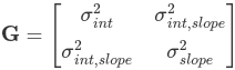

So far everything we've covered applied to both linear mixed models and generalized linear mixed models. What's different about these is that in GLMM the response variables can come from different distributions besides Gaussian. Additionally, rather than modeling the responses directly some link function (referred toi as g(.) and its inverse as h()) is often applied, such as log link. For example, in count outcomes are a special case in which we use a log link function and the probability mass function: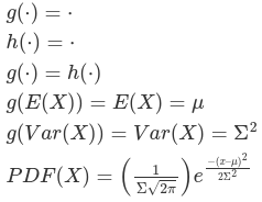

Interpretation

The interpretation of GLMMs is similar to GLMs. Often we want to transform our results to the original rather than the link function result;  this is where transformations complicate matters because they are nonlinear and so even random intercepts no longer. Consider the example below of a mixed effects logistic model predicting remission:

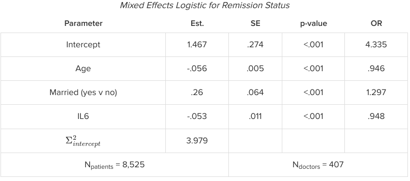
The estimates can be interpreted as always, where the estimated effect of the parameter is interpreted as a change in the log odds. However, we run into issues trying to interpret the odds ratios. Odds ratios take on a more complex meaning when there are mixed effects, as in a regular logistic model we assume all other effects are fixed. Thus we must interpret the odds ratio here as a conditional odds ratio for holding the remaining factors constant.

Estimation

For parameter estimation, there are no closed form solutions for GLMMs you must use some approximation

• Gaussian quadrature is a particularly well-suited method to numerically evaluate integrals against probability measures.
  • Suppose we have a probability density function p(x) and the function to be integrated against it f(x), the quadrature rule:
    

    

    where N denotes the number of quadrature points where w is the quadrature weights and x is the abscissas (locations).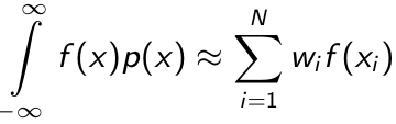
  • The Gaussian quadrature chooses abscissas in areas of high density, and if it is continuous the quadrille rule is exact is f(x) is a polynomial of up to degree 2R - 1
  • In the generalized linear mixed model the roles of f(x) and p(x) are played by the conditional distribution of the data given by the random effects and random effects distribution
  • Quadrature abscissas and weights are those of the standard Gauss-Hermite Quadrature
• Gauss-Hermite Quadrature is appropriate when the density is:
  

  

  • First we change the variables of integration to independent standard normal random effects v using the Cholesky decomposition L such that G = LL' so that b_i = Lv_i; We re-write the log likelihood:
    

    

    where phi(.) is the univariate standard normal density.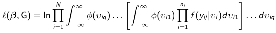
  • Each uni-dimensional integral can be approximated by Gauss-Hermite quadrature as:
    

    

    where sqrt(pi)*wr and ar/sqrt(2) are the weights and abscissas of the (2R-1)th degree Gauss-Hermite quadrature rule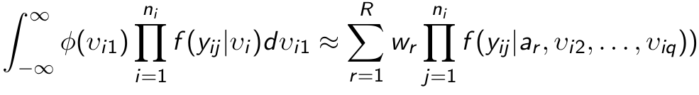
  • The approximation becomes more accurate as more quadrature points R are used.
  • This can be computationally expensive since the number of terms required to evaluate each multivariate integral is R^q

Gauss-Hermite quadrature has limitations; The number of function evaluations required grows exponentially as the number of dimensions increases. A random intercept is one dimension, adding a random slope would be two. For three level models with random intercepts and slopes, it is easy to create problems that are intractable with Gaussian quadrature. Consequently, it is a useful method when a high degree of accuracy is desired but performs poorly in high dimensional spaces, for large datasets, or if speed is a concern. Additionally, if the outcome is skewed there can also be problems with the random effects.

SAS Code

libname S857 'Z:\';

data amenorrhea;
set s857.amenorrhea;
t=time;
time2=time**2;
run;

proc sort data=amenorrhea;
by descending trt;
run;
title1 'Marginal Models';
title2 'Clinical Trial of Contracepting Women';

proc genmod data=amenorrhea descending;
class id trt (ref='0') t/param=ref;
model y = time time2 trt*time trt*time2 /dist=binomial link=logit type3 wald;
     repeated subject=id / withinsubject=t logor=fullclust;
store p1;
run;
ods graphics on;
ods html style=journal;
proc plm source=p1;
  score data = amenorrhea out=pred /ilink;
run;
proc sort data = pred;
  by trt time;
run;
proc sgplot data = pred;
  series x = time y = predicted /group=trt;
run;
ods graphics off;

title1 'Generalized Linear Mixed Effects Models';

proc glimmix  data=amenorrhea  method=quad(qpoints=5) empirical order=data ;
class id trt ;
model y = time time2 trt*time trt*time2 /dist=binomial link=logit s oddsratio;
random intercept time/subject=id type=un;
run;

title1 'Generalized Linear Mixed Effects Models';
title2 'Clinical Trial of AntiEpileptic-Drug';
data epilepsy;
set s857.epilepsy;
time=0;y=y0;output;
time=1;y=y1;output;
time=2;y=y3;output;
time=3;y=y3;output;
time=4;y=y4;output;
drop y0 y1 y2 y3 y4;
run;
data epilepsy;
set epilepsy;
if time=0 then t=log(8);
else t=log(2);
run;
proc sort data=epilepsy;
by descending trt;
run;
proc glimmix  data=epilepsy  method=quad(qpoints=50) empirical order=data ;
class id trt ;
model y = time trt trt*time /dist=poisson link=log s offset=t;
random intercept time/subject=id type=un;
run;
ods rtf close;