Response Profile Analysis

• Are the mean response profiles similar in the groups, or in other words, are the mean response profiles parallel?
  This is a question that concerns the group × time interaction effect
• Assuming that the mean response profiles are parallel, are the means constant over time?
  This is a question that concerns the time effect.
• Assuming that the mean response profiles are parallel, are they at the same level?
  This is a question that concerns the group effect.

Generalized Least Squares (GLS)

GLS is an extension of ordinary least squares (OLS) since it seeks to minimize a weighted sum of squared residuals. Unlike OLS, GLS accommodates heterogeneity and correlation via the weights which correspond to the inverse of the variance-covariance matrix. The parameters are estimated by minimizing the GLS objective function: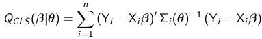

Theta is a vector of variance-covariance parameters. and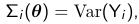  
We distinguish 2 cases, where theta is known and theta is not known.

Theta is Known

From calculus we know that in order to minimize the objective function we
1. Differentiate with respect to beta
2. Set the result to 0
3. Solve for beta
The solution to the minimization of the problem is: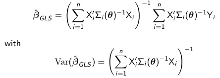

Since assuming we know the variance-covariance matrix of Y is a rather strong assumption we should protect ourselves against model mis-specification. We can use for inference the empirical "sandwich" estimator which is robust:

Theta is Unknown

When theta is unknown we need to replace it in the GLS formulas with a consistent estimate theta_hat. Typically theta_hat = theta_hat*beta_hat_0, where beta_hat_0 is an initial unbiased estimate of beta, such as the OLS estimate and theta_hat*beta_hat_0 is a non-iterative method of moments (MM) type estimator that is consistent for theta. Then the estimated generalized least squares estimator (ELGS) is: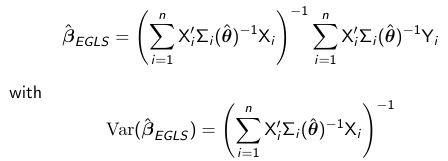

Maximum Likelihood

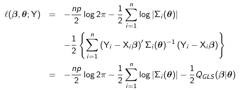
The most common approach to estimation is the method of maximum likelihood. The idea is to use an estimate of beta with the values that are most likely. Given that Y is assumed to have a conditional distribution that is multivariate normal we must maximize the following log-likelihood function:

Maximum Likelihood Estimators (MLE)

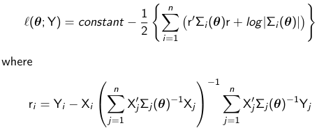
When theta is known and fixed the ML and GLS estimators are equivalent. When theta is unknown ML and EGLS estimators are equivalent if theta_hat (in EGLS) is equal to the ML estimate of theta. The MLE is estimated iteratively (as opposed to non-iteratively by EGLS) by maximizing the profile log-likelihood:

Variance of MLE

The variance of the MLE estimate beta_hat_MLE is: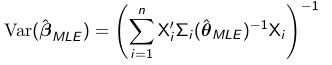

Similarly to GLS we can have a more robust "sandwich" estimator that can be used for inference:

Restricted Maximum Likelihood (REML)

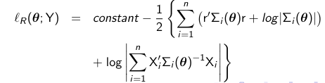
In small samples, ML estimation generally leads to small sample bias in the estimated variance components. To account for the fact that we have uncertainty from estimating beta, we can get unbiased estimates for the variance by maximizing the restricted profile log likelihood:

Variance of REML

Similar to other estimation procedures the variance of the REML estimate of beta_hat_REML is: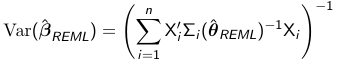

We also have a robust "sandwich" estimator that can be used for inference:

Inference

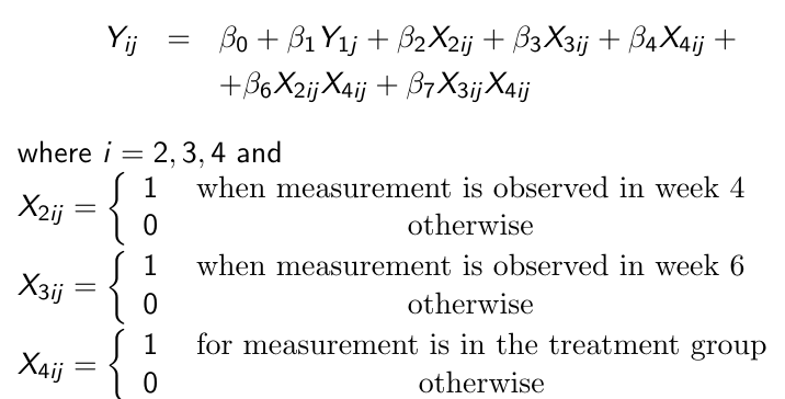
Consider the following linear representation of a response profile model: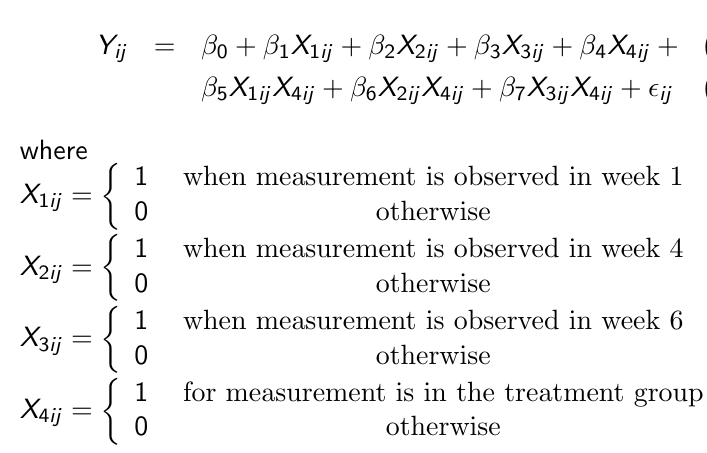

This gives us the following hypotheses:

1. Group x Time Interaction Effect
   Ex. H0: Beta_5, Beta_6, Beta 7 = 0 vs H1: At least one does not equal 0
2. Time Effect
   Ex. H0: Beta_1 = Beta_2 = Beta_3 vs H1: Beta_1, Beta_2, Beta_3 are not equal
3. Group Effect
   Ex. H0: Beta_4 = 0 vs H1: Beta_4 != 0

A large sample test for the general linear hypothesis:
    H0: L*Beta = 0; H1: L*Beta != 0
can be carried out using the Wald chi-square test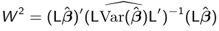

Where L is a r x p matrix of r contrasts or rank r <= p. If we want to test H0: Beta_5, Beta_6, Beta 7 = 0 for group*interaction effect: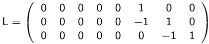

It can be shown that W² -> chi-squared(r) as n approaches infinity.

Another more robust approach is to replace var(beta_hat) with the robust sandwich estimator, var_r(beta_hat). However, there may be a loss in efficiency compared to the model-based estimator.

Contrasts from Baseline

In clinical trials, baseline response is independent from treatment, which means the groups have the same mean response at baseline. In this setting, we may be more interested in testing for equality of the difference between the average responses post-baseline and the baseline value in the two groups.

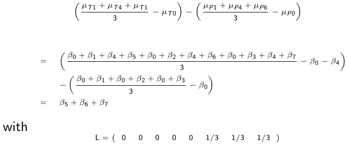
We can test it using the Wald test, which is W² -> chi²(1)

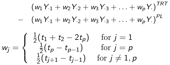
Area Under the Curve

Instead of comparing the difference of the average post-baseline responses, we can compare the area under the curve minus baseline (AUC). This corresponds to a calculation of the area under the trapezoidal curve.

Baseline as Covariate

An efficient way for testing group differences in a longitudinal clincal trial is to remove the baseline measure from the response and use it as a covariate in the post-baseline responses instead:

Strengths and Weaknesses

+ Is conceptually straightforward
+ It allows arbitrary patterns in the mean response over time
+ It allows for missing values in the response
+ There are various ways to adjust for the baseline

- Repeated measures must be obtained at the same sequence of time for all participants
- It ignores the time ordering of the repeated measures in a longitudinal study
- It may have low power to detect group differences in specific patterns of the mean response over time
- The number of estimated parameters grows rapidly with the number of measurement occasions