# Bayesian Logistic Regression
Let Y be an indicator for presence of disease -> Y | p ~ Bin(p, 1)
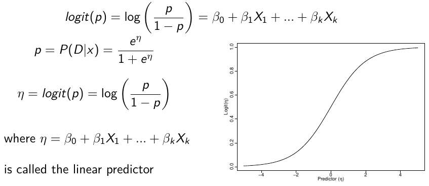
Logistic regression models the log-ODDS (also called logit) of the mean outcome using a linear predictor.
[](https://bookstack.mitchellhenschel.com/uploads/images/gallery/2023-01/2Rgimage.png)
[](https://bookstack.mitchellhenschel.com/uploads/images/gallery/2023-01/TCPimage.png)
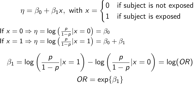
In a case-control study beta\_0 is not interpretable. But the estimate of log(OR) can be interpreted correctly, given the symmetry of roles of disease/exposure
H0: OR = 1; Log(OR) = 0; No association
H1: OR != 1; Log(OR) != 0; Significant association
The Frequentist approach to test the above is to fit a logistic regression in R using the function glm() and assess the OR.
In Bayesian formulation we need to identify the parameters in our prior model, and the parameters we wish to estimate to form a posterior distribution to assess the OR. We can compute the probability that OR > 1, < 1 or != 1 using a small range.
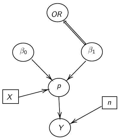
Ex. Below we model 2 parameters, beta\_0 and beta\_1, in a DAG model:
[](https://bookstack.mitchellhenschel.com/uploads/images/gallery/2023-01/9smimage.png)
Because there's no constraint on the beta regression parameters, it is common to assume a normal distribution.
The magnitude of variance reflects the amount of uncertainty
In the below code:
- We loop to specify each observation
- Y.D\[i\] =
- 1 if subject i has the disease
- 0 if subject i does not have the disease
- X.E\[i\] =
- 1 if subject i has been exposed
- 0 if subject i has not been exposed
```R
# Analysis with JAGS
library(rjags)
model.1 <- "model{
### data model
for(i in 1:N){
Y.D[i] ~ dbin(p[i], 1)
logit(p[i]) <- beta_0 + beta_1*X.E[i]
}
OR <- exp(beta_1)
pos.prob <- step(beta_1)
### prior
beta_1 ~ dnorm(0,0.0001)
beta_0 ~ dnorm(0,0.0001)
0 i th subject unexposed
}"
# In R Data stored as a list
data.1 <- list(N = 331, X.E = X.E, Y.D = Y.D)
# Compile model (data is part of it!); `adapt` for 2,000 samples
model_odds <- jags.model(textConnection(model.1), data = data.1,
n.adapt = 2000)
update(model_odds, n.iter = 5000) # 5,000 burn-in samples
# Get 10,000 samples from the posterior distribution of OR, beta_0,beta_1
test_odds <- coda.samples(model_odds, c("OR", "beta_1", "beta_0"), n.iter = 10000)
plot(test_odds)
summary(test_odds)
```
In the output, we'll often look for the point estimate to be the posterior mean. However, when posterior density is skewed, posterior median is sometimes preferable.
#### Asymptotic Approximation
When the sample size is large enough, one can use an asymptotic approximation of the posterior distribution of the parameters.
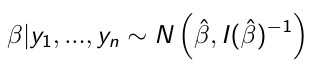
When the sampling distribution is a member of the exponential family (Normal, Binomial, Poisson, or Gamma), then the posterior distribution of the parameters is (approximately) normally distribution:
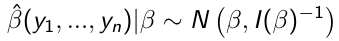
[\[1\]](https://bookstack.mitchellhenschel.com/uploads/images/gallery/2023-01/r6simage.png)
beta\_hat is the ML (maximum likelihood) estimate of beta
I(beta\_hat)^-1 is the Fisher Information matrix, evaluated in the ML estimate of beta
Based on the Maximum likelihood theory, asymptotically:
[\[2\]](https://bookstack.mitchellhenschel.com/uploads/images/gallery/2023-01/tssimage.png)
We don't need a prior in \[1\] because we have a lot of data. Results in \[1\] and \[2\] are close because the prior is weighted low because of the high sample size.
### Gibbs Sampling for Logistic Regression
[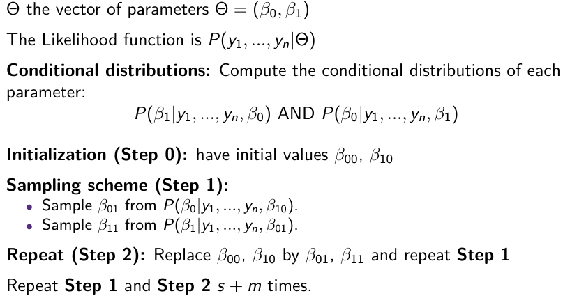](https://bookstack.mitchellhenschel.com/uploads/images/gallery/2023-01/woLimage.png)
##### Posterior Inference
Obtain s + m sample for each parameter
Throw away the first s values (burn-in)
Use the m samples with Monte Carlo algorithms to carry out inference:
1. Point Estimates - Posterior means or medians
[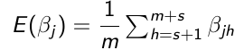](https://bookstack.mitchellhenschel.com/uploads/images/gallery/2023-01/HLmimage.png)
2. Transformations - Any function of the parameters
[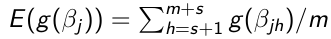](https://bookstack.mitchellhenschel.com/uploads/images/gallery/2023-01/TuPimage.png)
3. Posterior Density - Density estimation methods to estimate the posterior density of parameters
4. Tail probabilities
[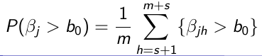](https://bookstack.mitchellhenschel.com/uploads/images/gallery/2023-01/9rDimage.png)
#### Marginal and Conditional Independence
Two random variables, X and Y, are independent (denoted by X ⊥ Y) if an only if:
P(X, Y) = P(X)P(Y); Joint p.m.f. for joint density = Marginal p.m.f. or marginal density
Given three random variables, X, Y and X, are conditionally independent given Z (denoted by Y ⊥ Y | Z) if and only if:
P(X, Y | Z) = P(X | Z) P(Y | Z)
There is no relation between marginal and conditional independence (Simpson Paradox)
The directed graph specifies conditional and marginal independence through two properties; The **Local Markov Property (LMP)** specifies that we need to specify only the distribution of nodes given their parents. The **Global Markov Property (GMP)** is used internally to derive the conditional distributions of each node given all others.
#### Local Markov Property (LMP)
Descendants of Y \[D(Y)\] are all nodes reached from Y with a directed path
Non-descendants of Y \[NS(Y)\] - all nodes minus the descendant nodes
[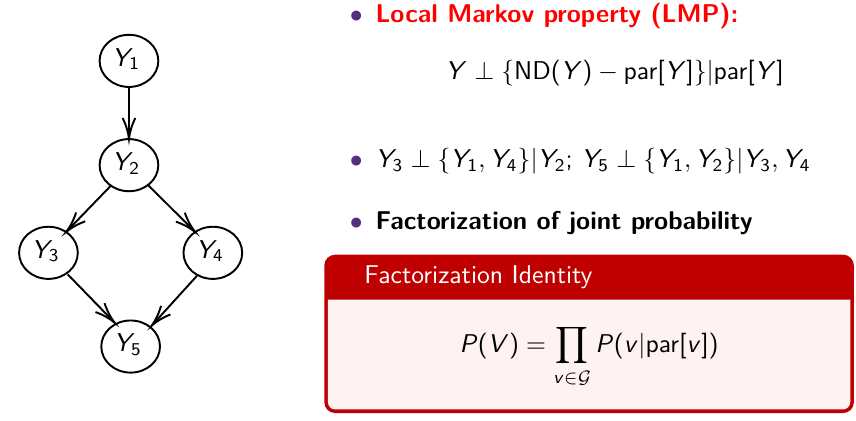](https://bookstack.mitchellhenschel.com/uploads/images/gallery/2023-01/IHMimage.png)
#### Global Markov Property (GMP)
The node is independent of everything else in the network given its Markov Blanket.
For each node, list the **Markov blanket:** Markov blanket of A: the parents of A, the children of A and the parents of the children of A
[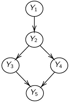](https://bookstack.mitchellhenschel.com/uploads/images/gallery/2023-01/5iqimage.png)
Y\_1 independent of Y\_3, Y\_4, Y\_5, given Y\_2
MB(Y\_1) = { Y\_2 }; MB(Y\_2) = { Y\_1, Y\_3, Y\_4 }
The LMP is used to specify the priors and the likelihood
The GMP is used to generate the conditional distributions to run the Gibbs Sampling
#### Bayesian Hypothesis Testing: Prior Odds
On each hypothesis we have a prior probability:
P(H0) = P(M0) and P(Ha) = P(M1)
Use the data to compute the posterior probability of each hypothesis:
[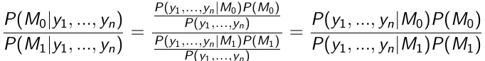](https://bookstack.mitchellhenschel.com/uploads/images/gallery/2023-01/cd5image.png)
This equates to:
Posterior ODDs = Bayes Factor \* Prior Odds
We accept the hypothesis with maximum posterior probability (0 - 1 loss)
The Bayes Factor is the ratio of the likelihood functions computed for models M0 and M1
If P(M0) = P(M1) then the posterior probability of M1 is larger than the posterior probability of M0
We can also assign weights to adjust the probability of making errors:
[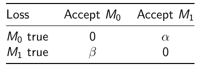](https://bookstack.mitchellhenschel.com/uploads/images/gallery/2023-02/image.png)
Where alpha would be the loss incurred if M1 is accepted when M0 is true
and beta is the loss incurred if M0 is accepted when M1 is true.