Propensity Score Weighting Analysis

Unlike randomized clinical trials, observational studies must adjust for differences such as confounding to ensure patient characteristics are comparable across treatment groups. This is frequently addressed through propensity scores (PS), which summarizes differences in patient characteristics between treatment groups. A Propensity Score is the probability that an individual will be assigned to receive the treatment of interest given their measured covariates. Matching or Weighting on the PS is used to adjust comparisons between the 2 groups, thus reducing the potential bias in estimated effects of observational studies.

The following use cases assume a binary treatment or exposure in order to infer causality. Given a treatment and control with one outcome observed per unit, can we estimate the treatment effect? Note we can only estimate the treatment effect, identification of causality is not possible through observational studies.

Note the following definitions before proceeding:

Target Population - The group of individuals who we wish to infer conclusions about
Balance - Similarity of patient characteristics across treatment
Precision - Denotes certainty about the estimate of association between treatment and outcome of interest; More precision means more narrow CIs and greater statistical power.

Estimation of Propensity Scores

Propensity scores are most commonly estimated using binomial regression models (logistic regression, probit, etc.). Other propensity score methods include:

Classification Trees
Bagging/Boosting
Neural Networks
Recursive Partitioning

Basically, any model that provides predictive probability and where all the covariates related to treatment and outcome that were measured before treatment are included in the propensity score estimation model. The SAS example below estimates propensity scores for the treatment variable group predicted from covariates var1, var2, and var3 using a logistic regression:

PROC LOGISTIC data=ps_est;
  title 'Propensity Score Estimation';
  model exposure = var1-var3 / lackfit outroc = ps_r;
  output out = ps_p pred = ps xbeta=logit_ps;
  /* Output the propensity score and the logit of the propensity score */
run;

Once we have the propensity scores estimated, we must make sure the measured covariates are balanced in order to reduce bias. There are several ways to achieve this:

Graphic of the propensity score distribution - The distribution of propensity score between the two groups should overlap. Non-overlapping distributions suggest that one or more covariates are strongly predictive, and variable selection or stratification should be reconsidered.
Standardized differences of each covariate between treatment groups - the magnitude of the difference between baseline characteristics of the groups can be calculated depending on the method of deriving propensity scores. One limitation of this method is the lack of consensus as to what the threshold should be, though researchers have suggested a standardized difference of .1 or more denotes meaningful imbalance in the baseline covariates.
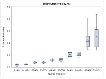
Stratify by deciles or quintiles (5 parts) - By stratifying the propensity score by deciles or quintiles, a boxplot can represent each quintile.

When the scores aren't balanced, the covariates in the model should be adjusted. This could mean adding or removing covariates, adding interactions, or substituting a non-linear term for a continuous one.

Covarite Balancing Propensity Scores

After we obtain the propensity score, the next step is to estimate the Average Treatment Effect in the population (ATE). Using multiple methods can help strengthen conclusions, while discrepancies can indicate confounding and/or sensitivity to the analysis approach.

A key diagnostic is the standardized mean difference (SMD)- The normalized difference in means between two groups for a given covariate. A SMD score of > .1 for a given covariate generally indicates imbalance.

Stratification

Stratification divides individuals into many groups on the basis of their propensity score values. The optimal number of strata depends on sample size and the amount of overlap between treatment and control group propensity scores, however researchers have suggested 5 subclasses is sufficient enough to remove 90% of bias in the majority of PS studies. The treatment effect for each subclass is the average effect across strata weighted by stratum-specific standard error:

$$ \hat\mu_{1i} - \hat\mu_{2i} = {{\sum w_i (\bar X_{1i} - \bar X_{2i}) } \over {\sum w_i}} $$

Where $ w_i = { 1 \over {SE}^2_i} $ (the square of the standard error of the difference between means). This can be coded in SAS as follows:

/* Stratify */
PROC RANK data=ps_p out=ps_strata groups=5;
	var ps_pred;
    ranks ps_pred_rank;
run;

/* Sort */
proc sort data = ps_strataranks;
	by ps_pred_rank;

/* Compute the difference between group means in each stratum,
	as well as the standard error of this within stratum difference */
proc ttest;
  by ps_pred_rank;
  class group;
  var outcome;
  ods output statistics = strata_out;

/* Find stratum specific weights and mutliply by mean difference */
data weights;
  set strata_out;
  if class = 'Diff (1-2)';
  wt_i = 1/(StdErr**2);
  wt_diff = wt_i*Mean;
 
/* Find the mean weighted difference and its standard error */
proc means noprint data = weights;
  var wt_i wt_diff;
  output out = total sum = sum_wt sum_diff;
  data total2;
  set total;
  Mean_diff = sum_diff/sum_wt;
  SE_Diff = SQRT(1/sum_wt);

proc print data = total2;

run;

Matching

The goal of matching is to obtain similar groups of treatment and control subjects by matching individual observations on their propensity scores. It is generally recommended to use 1:1 matching with no replacement to avoid bias. The Nearest Neighbor (or Greedy matching) selects a control unit for each treated unit based on the smallest distance from the treated unit. The big problem with this is it depends on the order in which the data is sorted, thus randomization is necessary.

Nearest Neighbor with calipers is a method which improves NN by allowing a maximum allowable difference between scores (or caliper width) in order for PS to be matched. Researchers have suggested a caliper width of .2 times the standard deviation, or a static value such as .1.

The general procedure:

Sort observations into random order with each group
Transpose data to obtain seperate datasets for treatment and control
Merge them into a single dataset, matching each observation in the treatment group with a single observation in the control group
- If no control observations are found in the range, no matched pair is created
After matched pairs have been identified, the difference in outcome means in each group can be tested ussing a t-test.
- Use a correlated-means t-test rather than independant-means (PAIRED keyword in SAS)

/* Use the propensity score model probabilities to match case and control 1:1 */
proc psmatch data=ps_p region=cs;
  class exposure;
  psmodel exposure = var1-var3;
  match distance=lps method=greedy(k=1) stat=lps caliper(mult=stddev)=.15;
  assess lps var=(var1-var3)/weight=none plots=(boxplot);
  output out(obs=match)=match1 lps=_Lps matchid=_MatchId;
run;

Inverse Probability of Treatment Weights (IPTW)

In IPTW, individuals are weighted by the inverse probability of receiving the treatment they actually received. So, the target estimand is the treatment effect in the treated population. Control subjects are weighted by $1 / (1 - p_i) $ and treated subjects with $ 1/p_i $. The weights are then used in a Weighted Least Squares regression model.

data ps_weight;
  set ps_p;
  if group = 1 then ps_weight = 1/ps_pred;
  else ps_weight = 1/(1-ps_pred);
run;

proc means noprint data = ps_weight;
  var ps_weight;
  output out = q mean = mn_wt;
run;

data ps_weight2;
  if _n_ = 1 then set q;
  retain mn_wt;
  set ps_weight;
  wt2 = ps_weight/mn_wt; * Normalized weight;
run;

/* Either of the below can be used to estimate treatment effect
 via weighted least sqaures */
proc glm data = ps_weight2;
  class group;
  model outcome = group / ss3 solution;
  weight wt2;
  means group;
run;

proc reg data = ps_weight2;
  model outcome = group;
  weight wt2;
run

The IPTW method is inclusive of all subjects, so no data loss occurs. However, it is very sensitive to outliers and can create extreme weights. There exist stabilization techniques which use trimming or scaling to get weights into a specified range.

Overlap Weighting

Overlap weighting (OW) is a new PS method aimed to address the shortcoming of IPTW. In IPTW, individuals are weighted by the inverse probability of being in their treatment group, which allowed under-representing characteristics to count more. In OW, patients are assigned weights which are proportional to the probability of that patient belonging to the other treatment group. That is, treated patients are given a weight of (1 - PS) while non-treated are weighted by the probability of treatment PS. The target estimand is the average treatment effect for the overlap population.

These weights are smaller for extreme values so outliers are treated as PS near 1 or 0, and do not dominate or worsen precision as with IPTW. Patients whose characteristics are compatible with either group contribute relatively more. The result can be as efficient as randomization. Overlap weighting creates an exact balance on the mean of every measured covariate when the PS is estimated by logistic regression. This is advantageous when groups being compared are initially very different.

We can use the code from IPTW replacing the weight of 1/PS with 1 - PS in the treated group and 1/(1-PS) with PS in the untreated group. Note that adjustments such as trimming have nearly no effect on the weighted balance of OW.

* Generating overlap wieghts;
data overlap;
  set ps_p;
  ow_weight = (EXPOSURE)*(1-ps) + (1 - EXPOSURE)*ps;
run;

* then normalize it;

Estimating Treatment Effect

With the generated weights or matched dataset pick a fitting model to determine the effects of the exposure on the outcome of interest. If any covariates remain imbalanced, they can be included in the model. Otherwise, the model should only contain outcome and exposure.

* Continous Outcome;
proc glm data=overlap2;
  class exposure(ref="0");
  model OUTCOME = EXPOSURE/solution;
  weight ow_weight;
run;

* Dichotomous outcome (in this case coded into several binary variables);
proc genmod data=overlap2;
  class exposure(ref="0");
  model OUTCOME1 = EXPOSURE/dist=BINOMIAL;
  weight ow_weight;
run;

R

The above code examples use SAS to explain the underlying concepts. There are several R packages that can provide propensity score weighting with binary treatments, but the newest and most popular is PSweights. I recommend checking out the documentation and whitepaper (link below) to understand the functionalities this package can provide.