Advanced Machine Learning
Recall that in an ordinary multiple linear regression, we have a set of p predictor variables measuring some response variable (Y) to fit a model like:
$$ Y = \beta_0 + \beta_1 X_1 ... \beta_p X_p + \epsilon $$
Where beta represents the average effect of a unit increase in the predictor Xn (the nth predictor variable) and epsilon is the error term. The value for these beta coefficients is chosen using the least square method, which minimizes the sum of squared residuals (RSS), or the squared difference in observed minus expected outcome value.
$$ RSS = \Sigma (y_i - \hat y_i)^2 $$
Least Absolute Shrinkage and Selection Operator (LASSO)
When variables are highly correlated then coefficient estimates can have large variances leading to poor predictive accuracy.
Lasso regression is a regularization technique for linear regression models. Regularization is a statistical method to reduce errors caused by overfitting on training data. Instead of trying to minimize RSS, Lasso uses the equation:
Total Cost = Measure of Fit [RSS] + Measure of magnitude of coefficients
$$ Cost = RSS + \lambda \Sigma | \beta_n | ; \lambda \ge 0 $$
Lambda is the 'tuning' parameter, or shrinkage penalty, and measures the balance of fit and sparsity. When this term is 0 the parameter has no effect, and as it approaches infinity the shrinkage penalty becomes more influential.
- Start with full model (all possible features)
- "Shrink" some coefficients to 0 (exactly)
- Non-zero coefficients indicate "selected" features
The idea is to have as little bias as possible so the variance can be reduced, leading to a smaller mean squared error (MSE).
Note: This is very similar to ridge regression, except in ridge the coefficients are minimized toward 0 but must always be > 0
Lasso tends to perform better when only a small number of predictor variables are significant, and ridge when all coefficients have roughly equal importance. To determine which model is better use k-fold cross validation.
Process
- Calculate correlation matrix and variance inflation factor values (VIF) for all predictor variables
- Fit the lasso regression model and choose a value for lambda
- Compare to a another regression model by way of k-fold cross-validation
Code
# https://www.r-bloggers.com/2020/05/quick-tutorial-on-lasso-regression-with-example/

library(glmnet)
# Loading the data
data(swiss)
x_vars <- model.matrix(Fertility~. , swiss)[,-1]
y_var <- swiss$Fertility
lambda_seq <- 10^seq(2, -2, by = -.1)
# Splitting the data into test and train
set.seed(86)
train = sample(1:nrow(x_vars), nrow(x_vars)/2)
x_test = (-train)
y_test = y_var[x_test]
cv_output <- cv.glmnet(x_vars[train,], y_var[train],
                       alpha = 1, lambda = lambda_seq,
                       nfolds = 5)
# identifying best lamda
best_lam <- cv_output$lambda.min
best_lam


# Output
# [1] 0.3981072


# Rebuilding the model with best lamda value identified
lasso_best <- glmnet(x_vars[train,], y_var[train], alpha = 1, lambda = best_lam)
pred <- predict(lasso_best, s = best_lam, newx = x_vars[x_test,])
# Combine predicted and actual values
final <- cbind(y_var[test], pred)
# Checking the first six obs
head(final)


# Output
#            Actual    Pred
#Courtelary   80.2 66.54744
#Delemont     83.1 76.92662
#Franches-Mnt 92.5 81.01839
#Moutier      85.8 72.23535
#Neuveville   76.9 61.02462
#Broye        83.8 79.25439


# R-squared
actual <- test$actual
preds <- test$predicted
rss <- sum((preds - actual) ^ 2)
tss <- sum((actual - mean(actual)) ^ 2)
rsq <- 1 - rss/tss
rsq


# Inspecting beta coefficients
coef(lasso_best)


# Output
#6 x 1 sparse Matrix of class "dgCMatrix"
#                         s0
#(Intercept)      66.5365304
#Agriculture      -0.0489183
#Examination       .
#Education        -0.9523625
#Catholic          0.1188127
#Infant.Mortality  0.4994369
XGBoost
XGBoost is a software library installed independently from whatever language is used to interact with it. Most popular languages have an interface, and there is a CLI version.
The library is focused on computational speed and model performance, and there are a number of advanced features. As the name suggests it uses a model optimization technique called gradient boosting, or gradient tree boosting. Let's quickly review.
Gradient Boosting
The original paper: Greedy Function Approximation: A Gradient Boosting Machine [PDF], 1999
The objective is to minimize the loss of the model by adding 'weak learners' ( usually a decision tree) using a gradient-descent like procedure. It is considered a stage-wide additive model, and was the landmark in the use of differentiable loss functions. The technique could be applied beyond binary classification problems to regression, multi-class classification models and more.
How it works:
1. A loss function to be optimized
This depends on the type of problem being solved. In the case of a regression one may used squared error (RSS), and a classification problem might have a logarithmic loss.
The benefit of gradient boosting is it does not need to derive a new boosting algorithm for each loss function; it is generic enough that any differentiable function can be used.
2. A decision tree to make predictions
Specifically regression trees that output real values for model outputs. This allows subsequent model outputs to be added together, and 'correct' the residuals.
Trees are constructed in a greedy manner, choosing best split points based on purity scores (e.g. Gini index) to minimize the lost. It is common to constrain the tree in specific ways, such as max nodes, layers, splits, or leaf nodes.
3. An additive model to add weak learners to minimize the loss function
A gradient descent procedure is used to minimize the loss when adding trees.
Traditionally, gradient descent is used to minimize a set of parameters. Error or loss is calculated and weights are updated to minimize that error.
Instead of parameters we have decision tree regression models. After calculating the loss in a given model, we must add the tree/model that reduces the loss (i.e. follow the gradient). This is done by parameterizing the tree then modifying the parameters of the tree to move in the right direction by reducing the residual loss. The output of the new tree is then added to the existing sequence of trees in an effort to correct the final output of the model.
A fixed number of trees are added or training stops once loss reaches an acceptable level or no longer improves based on the validation set.
Common Enhancements to Gradient Boosting
- Tree Constraints - As mentioned above, constraints on number of leaves, nodes, etc.
- Shrinkage/Weighted Updates - The predictions of each tree are added together sequentially and the contribution of each tree added can be weighted to 'slow down' the learning algorithm.
- Random sampling/Stochastic Gradient Boosting - Instead of using the full dataset, at each iteration a sub-sample of the training data is used (without replacement) to fit the base learner.
- Penalized learning/Regularized Gradient Boosting - The decision trees can be made more complex by adding regularization terms (often called weights) to smooth the final learnt weights to avoid over-fitting. By design this tends to select a simple and predictive model.
XGBoost Features
XGBoost supports all of the above common enhancements. In addition the software library can run distributed, parallel, out-of-core, and with cache optimization to make best use of hardware. Additionally, it can automatically handle missing data and provide continued training for new data.
Even with all these cool features XGBoost will only take numeric data as input. Code your character inputs to factors to create a matrix.
I'm going to include a list of hyperparameters below; These provide a simple interface for complicated tuning variables.
Full reference: https://xgboost.readthedocs.io/en/latest/parameter.html
| Parameter | Explanation |
|---|---|
| eta | default = 0.3 learning rate / shrinkage. Scales the contribution of each try by a factor of 0 < eta < 1 |
| gamma | default = 0 minimum loss reduction needed to make another partition in a given tree. larger the value, the more conservative the tree will be (as it will need to make a bigger reduction to split) So, conservative in the sense of willingness to split. |
| max_depth | default = 6 max depth of each tree… |
| subsample | 1 (ie, no subsampling) fraction of training samples to use in each “boosting iteration” |
| colsample_bytree | default = 1 (ie, no sampling) Fraction of columns to be used when constructing each tree. This is an idea used in RandomForests |
| min_child_weight | default = 1 This is the minimum number of instances that have to been in a node. It’s a regularization parameter So, if it’s set to 10, each leaf has to have at least 10 instances assigned to it. The higher the value, the more conservative the tree will be. |
Once you have your boosting model prepared run xgb.train()and xgboost()to train the boosting model. Both return a wrapper of class xgb.Booster, but xgb.train is an advanced interface which xboost is a simple wrapper for the former.
One of the parameters set in xgboost()is nrounds - the max number of boosting iterations (AKA how many decision trees get added). Setting this too low will result in a model which is too simple, and setting it too high leads to overfitting. The goal is to find the middle ground.
We should cross-validate to determine the correct numbe of rounds and other hyperparameters. XGBoost has a function to do this for us: xgb.cv()
Code
# https://www.r-bloggers.com/2020/10/an-r-pipeline-for-xgboost-part-i/
# https://www.kaggle.com/c/titanic/data
#
library(xgboost)
library(Matrix)
library(xgboost)
library(ggplot2)
library(ggthemes)
library(readr)
library(dplyr)
library(tidyr)
library(stringr)
theme_set(theme_economist())
set.seed(1234) # For reproducibility.

directoryWhichContainsTrainingData <-  "./xg_boost_data/train.csv"
directoryWhichContaintsTestData <- "./xg_boost_data//test.csv"

titanic_train <- read_csv(directoryWhichContainsTrainingData)
titanic_test <- read_csv(directoryWhichContaintsTestData)

titanic_train <- titanic_train %>%
  select(Survived,
         Pclass,
         Sex,
         Age,
         Embarked)

titanic_test <- titanic_test %>%
  select(Pclass,
         Sex,
         Age,
         Embarked)

str(titanic_train, give.attr = FALSE)
## tibble [891 x 5] (S3: tbl_df/tbl/data.frame)
##  $ Survived: num [1:891] 0 1 1 1 0 0 0 0 1 1 ...
##  $ Pclass  : num [1:891] 3 1 3 1 3 3 1 3 3 2 ...
##  $ Sex     : chr [1:891] "male" "female" "female" "female" ...
##  $ Age     : num [1:891] 22 38 26 35 35 NA 54 2 27 14 ...
##  $ Embarked: chr [1:891] "S" "C" "S" "S" ...

previous_na_action <- options('na.action') #store the current na.action
options(na.action='na.pass') #change the na.action

titanic_train$Sex <- as.factor(titanic_train$Sex)
titanic_train$Embarked <- as.factor(titanic_train$Embarked)

#create the sparse matrices
titanic_train_sparse <- sparse.model.matrix(Survived~., data = titanic_train)[,-1]
titanic_test_sparse <- sparse.model.matrix(~., data = titanic_test)[,-1]

options(na.action=previous_na_action$na.action) #reset the na.action

str(titanic_train_sparse)
## Formal class 'dgCMatrix' [package "Matrix"] with 6 slots
##   ..@ i       : int [1:3080] 0 1 2 3 4 5 6 7 8 9 ...
##   ..@ p       : int [1:6] 0 891 1468 2359 2436 3080
##   ..@ Dim     : int [1:2] 891 5
##   ..@ Dimnames:List of 2
##   .. ..$ : chr [1:891] "1" "2" "3" "4" ...
##   .. ..$ : chr [1:5] "Pclass" "Sexmale" "Age" "EmbarkedQ" ...
##   ..@ x       : num [1:3080] 3 1 3 1 3 3 1 3 3 2 ...
##   ..@ factors : list()

dim(titanic_train_sparse)
## [1] 891   5
head(titanic_train_sparse@Dimnames[[2]])
## [1] "Pclass"    "Sexmale"   "Age"       "EmbarkedQ" "EmbarkedS"

# booster = 'gbtree': Possible to also have linear boosters as your weak learners.
params_booster <- list(booster = 'gbtree', eta = 1, gamma = 0, max.depth = 2, subsample = 1, colsample_bytree = 1, min_child_weight = 1, objective = "binary:logistic")

# NB: keep in mind xgb.cv() is used to select the correct hyperparams.
# Here I'm only looking for a decent value for nrounds; We won't do full hyperparameter tuning.
# Once you have them, train using xgb.train() or xgboost() to get the final model.

bst.cv <- xgb.cv(data = titanic_train_sparse,
              label = titanic_train$Survived,
              params = params_booster,
              nrounds = 300,
              nfold = 5,
              print_every_n = 20,
              verbose = 2)

# Note, we can also implement early-stopping: early_stopping_rounds = 3, so that if there has been no improvement in test accuracy for a specified number of rounds, the algorithm stops.

res_df <- data.frame(TRAINING_ERROR = bst.cv$evaluation_log$train_error_mean,
                     VALIDATION_ERROR = bst.cv$evaluation_log$test_error_mean, # Don't confuse this with the test data set.
                     ITERATION = bst.cv$evaluation_log$iter) %>%
  mutate(MIN = VALIDATION_ERROR == min(VALIDATION_ERROR))

best_nrounds <- res_df %>%
  filter(MIN) %>%
  pull(ITERATION)

res_df_longer <- pivot_longer(data = res_df,
                              cols = c(TRAINING_ERROR, VALIDATION_ERROR),
                              names_to = "ERROR_TYPE",
                              values_to = "ERROR")

g <- ggplot(res_df_longer, aes(x = ITERATION)) +        # Look @ it overfit.
  geom_line(aes(y = ERROR, group = ERROR_TYPE, colour = ERROR_TYPE)) +
  geom_vline(xintercept = best_nrounds, colour = "green") +
  geom_label(aes(label = str_interp("${best_nrounds} iterations gives minimum validation error"), y = 0.2, x = best_nrounds, hjust = 0.1)) +
  labs(
    x = "nrounds",
    y = "Error",
    title = "Test & Train Errors",
    subtitle = str_interp("Note how the training error keeps decreasing after ${best_nrounds} iterations, but the validation error starts \ncreeping up. This is a sign of overfitting.")
  ) +
  scale_colour_discrete("Error Type: ")

g

bstSparse <- xgboost(data = titanic_train_sparse, label = titanic_train$Survived, nrounds = best_nrounds, params = params_booster)
## [1]  train-error:0.207632
## [2]  train-error:0.209877
## [3]  train-error:0.189675
## [4]  train-error:0.173962
## [5]  train-error:0.163861
## [6]  train-error:0.166105
## [7]  train-error:0.166105
## [8]  train-error:0.162739
## [9]  train-error:0.156004

titanic_test <- read_csv(directoryWhichContaintsTestData)

predictions <- predict(bstSparse, titanic_test_sparse)
titanic_test$Survived = predictions

titanic_test <- titanic_test %>% select(PassengerId, Survived)
titanic_test$Survived = as.numeric(titanic_test$Survived > 0.5)
Support Vector Machine (SVM)
SVMs, AKA vector networks, are supervised max-margin models for classification and regression analysis. The concept is very easy to understand; We use data labels to generate multiple separating regions (called hyperplanes) that separate the data points.
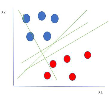
The goal is to maximize the margin, so that both groups of points are equidistant from the plane that divides them.
Hard margins are typically referred to as linear lines that can separate the data. Of course, this is a vast oversimplification. In reality, data is rarely linearly separable. Soft margins must be used to allow for weaker boundaries. This is where the support vector machine comes in.
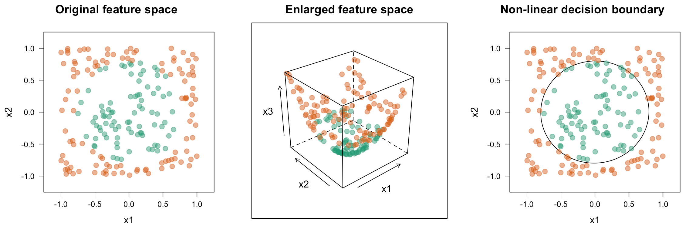
To adapt to nonlinear relationships SVM uses a kernel function. This is a mathematical function used to map input data into a high-dimensional feature space. Common kernel functions include:
- Linear AKA dot product - K(x, xi) = sum(x * xi)
- Polynomial - K(x,xi) = 1 + sum(x * xi)^d; When d=1 this is the same as linear regression. Manually setting d allows for curved lines in the input space
- Radial basis function - K(x,xi) = exp(-gamma * sum((x – xi^2)); Good for complex polygons
- & more
A key player in the kernel function are the support vectors, vectors which contain the data points closest to the hyperplane which divides the data.
This gives SVMs with proper training data a high predictive accuracy for classification tasks. However, one downside is there is no 'probability' in the sense of how effective a prediction is.
Code
dataset = read.csv('Social_Network_Ads.csv')
dataset = dataset[3:5]

# Encoding the target feature as factor
dataset$Purchased = factor(dataset$Purchased, levels = c(0, 1))

# Splitting the dataset into the Training set and Test set
install.packages('caTools')
library(caTools)

set.seed(123)
split = sample.split(dataset$Purchased, SplitRatio = 0.75)

training_set = subset(dataset, split == TRUE)
test_set = subset(dataset, split == FALSE)

dat = data.frame(x, y = as.factor(y)) # make output a factor
library(e1071) # contains svm function

classifier = svm(formula = Purchased ~ .,
                 data = training_set,
                 type = 'C-classification',
                 kernel = 'linear',
                 scale = TRUE) # do not scale
print(classifier)
plot(classifier, dat)


# Predicting the Test set results
y_pred = predict(classifier, newdata = test_set[-3])

# Making the Confusion Matrix
cm = table(test_set[, 3], y_pred)
No Comments