Poisson Regression

We use the Poisson Regression to model a risk ratio when we are interested not in whether something occurs but how many times it occurs; Either repeated events or events in a population.Ex. number of hospitalizations, number of infections, etc.

Logistic regression produces odd ratios (which approximates risk ratio when outcome is rare), but only analyzes patients with at least 1 event and can be difficult to interpret when outcome is not rare. Survival analysis can be used to analyze the time to the first event.

Poisson Distribution

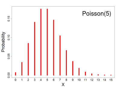
X ~ Poisson(μ); μ > 0
X = the number of occurrences of an event of interest, with parameter μ
Probability mass function
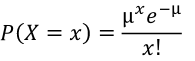
E(X) = μ
V(X) = μ

The distribution depends of the expected number of events, since the mean = variance. As the number of expected number of events increases it the more closely the Poisson distribution approximates the normal distribution.

If X ~ Binomial(n, p) and n -> inf, p -> 0 such that np is constant; X ~ Poisson(np)

Distribution of the sum of independent Poisson random variables. If Xi ~ Poisson(μi) for i = 1 to m, and teh Xi's are independent then: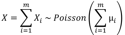

IR = (number of events)/(number of controls OR interventions)
Incident Rate Ratio = IR_intervention / IR_controls

CI for expected number of events (μ):
μ_L, μ_U = X +/- 1.96 * sqrt(X)

CI for Incidence Rate: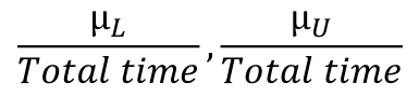

The event rate can also be written as:
λ = μ / N
Where μ is the expected number of events and N is the number of exposure units

We model the relationship on the log scale: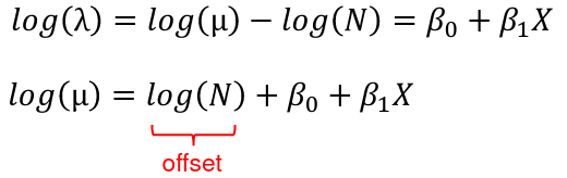

So to use the Poisson model we need 3 things:

Predictor variables and covariates X1, X2, X3...
The number of events for each "subject", defined as the group to which the event count belongs
The denominator that the events are drawn from Ni

For specific values of X, X*, X+:

For a CI for IRR(X* vs X+):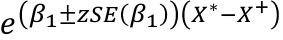

library(epitools)
library(aod) # For Wald tests
library(MASS) # for glm.nb()
library(lmtest) # for lrtest()
library(gee) # for gee()
library(geepack) # for geeglm()

## Poisson regression
### Import data
patients <- read.csv("patients.csv", header=T)


### Poisson regression: crude model
mod.p <- glm(NumEvents ~ Intervention, family = poisson(link="log"), offset = log(fuptime), data=patients)
summary(mod.p)
confint.default(mod.p)
exp(cbind(IRR = coef(mod.p), confint.default(mod.p))) 

### Poisson regression: adjusted model
mod.p2 <- glm(NumEvents ~ Intervention + Severity, family = poisson(link="log"), offset = log(fuptime), data=patients)
summary(mod.p2)
exp(cbind(IRR = coef(mod.p2), confint.default(mod.p2))) 

### Poisson regression with summary data
Intervention <- c(0,1)
NumEvents <- c(481,463)
fuptime <- c(876,1008)

mod.s <- glm(NumEvents ~ Intervention, family = poisson(link="log"), offset = log(fuptime))
summary(mod.s)
exp(cbind(IRR = coef(mod.s), confint.default(mod.s))) 

## Overdispersed data
d <- read.csv("overdispersion.csv", header=T)

mod.o1 <- glm(n_c ~ as.factor(region) + as.factor(age), family = poisson(link="log"), offset = l_total, data=d)
summary(mod.o1)
# Joint tests:
## Test of region
wald.test(b = coef(mod.o1), Sigma = vcov(mod.o1), Terms = 2:4)
## Test of age
wald.test(b = coef(mod.o1), Sigma = vcov(mod.o1), Terms = 5:6)

# Estimate dispersion parameter using pearson residuals
dp = sum(residuals(mod.o1,type ="pearson")^2)/mod.o1$df.residual
# Adjust model for overdispersion:
summary(mod.o1, dispersion=dp)


# Estimate dispersion parameter using deviance residuals
dp2 = sum(residuals(mod.o1,type ="deviance")^2)/mod.o1$df.residual
# Adjust model for overdispersion:
summary(mod.o1, dispersion=dp2)

### Adjust for overdispersion using quasipoisson
mod.o2 <- glm(n_c ~ as.factor(region) + as.factor(age), family = quasipoisson(link="log"), offset = l_total, data=d)
summary(mod.o2)
## Test of region
wald.test(b = coef(mod.o2), Sigma = vcov(mod.o2), Terms = 2:4)
## Test of age
wald.test(b = coef(mod.o2), Sigma = vcov(mod.o2), Terms = 5:6)

### Negative Binomial regression
# Note the offset is now added as a variable
# Allow for up to 100 iterations
mod.o3 <- glm.nb(n_c ~ as.factor(region) + as.factor(age) + offset(l_total), control=glm.control(maxit=100), data=d)
summary(mod.o3)
## Test of region
wald.test(b = coef(mod.o3), Sigma = vcov(mod.o3), Terms = 2:4)
## Test of age
wald.test(b = coef(mod.o3), Sigma = vcov(mod.o3), Terms = 5:6)

### LRT to compare Poisson and Negative Binomial models
lrtest(mod.o1, mod.o3)

# Not this:
anova(mod.o1, mod.o3)

## Risk Ratio regression
ACE <- read.csv("BU Alcohol Survey Motives.csv", header=T)

oddsratio(table(ACE$OnsetLT16, ACE$AUD), rev='both', method='wald')

riskratio(table(ACE$OnsetLT16, ACE$AUD), method='wald')

### Log-Binomial model
# Crude
mod.lb1 <- glm(AUD ~ OnsetLT16, family = binomial(link="log"), data=ACE)
summary(mod.lb1)
exp(cbind(RR = coef(mod.lb1), confint.default(mod.lb1))) 

# Adjusted (did not converge)
#mod.lb2 <- glm(AUD ~ OnsetLT16 + as.factor(Sex) + as.factor(ACEcat3) + Age, family = binomial(link="log"), data=ACE)

### Modified Poisson
# Crude using gee()
mod.mp1 <- gee(AUD ~ OnsetLT16, id=id, family = poisson(link="log"), data=ACE)
summary(mod.mp1)

# Crude using geeglm()
mod.mp1.2 <- geeglm(AUD ~ OnsetLT16, id=id, family = poisson(link="log"), data=ACE)
summary(mod.mp1.2)

# Adjusted using gee()
mod.mp2 <- gee(AUD ~ OnsetLT16 + as.factor(Sex) + as.factor(ACEcat3) + Age, id=id, family = poisson(link="log"), data=ACE)
summary(mod.mp2)

# Adjusted using geeglm()
mod.mp2.2 <- geeglm(AUD ~ OnsetLT16 + as.factor(Sex) + as.factor(ACEcat3) + Age, id=id, family = poisson(link="log"), data=ACE)
summary(mod.mp2.2)