Power and Sample Size Calculations for Association Studies

Review of errors and difference in means/proportions: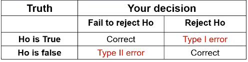

Type II error is represented by beta and type I error as alpha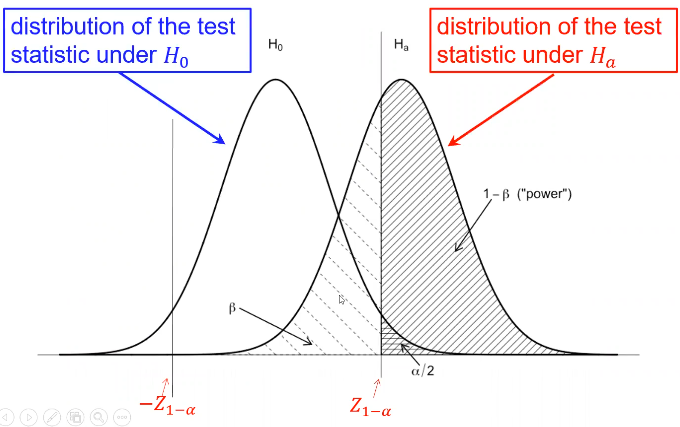

Where Z_{1 - (alpha /2)}is the Z-value that creates the target value of alpha in the tail of the distribution. Power decreases as alpha increases.

Power also has a direct relationship with sample size. Sometimes we choose sample sized based on the desired power for a specific alternative hypothesis of interest, and other times we used a fixed sample size and significance level.

A Z-test of differences in proportions with 2 groups with different sample sizes: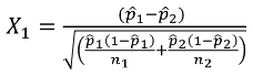

C is the mean of the distribution under the alternative hypothesis: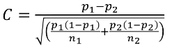

And the power can be calculated by taking the cdf of C minus the one sided Z-value

Likewise, we can use a similar z-test for differences in the mean of a quantitative trait: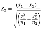

And the power can be calculated the same way as proportions.

Applying Power to Genetic Associations

• Difference in proportions: we can compute the power for a test that  compares the allele or genotype frequency between cases and controls
• Difference in means: we can compare the mean trait values between individuals with different genotypes at a marker (and we can extend this to an F-test for a linear regression)

Dichotomous Traits

1. Determine the expected genotype frequencies in cases and controls under the alternative hypothesis of interest
2. Estimate power for given sample size or estimate minimum sample size required for given power and significance level under the planner analysis model

Genetic Model

• We usually use 4 parameters to specify the disease model for a dichotomous trait:
  • Genotype relative risks y₁ and y₂
  • Population prevalence of disease K
  • Risk allele frequency q (the allele that increases risk of disease)
• To compute power, we need the genotype frequencies for cases and controls under the alternative hypothesis
  • P(personal carries i risk alleles | affected)
  • P(Person carries i risk alleles | unaffected)
  • for i = 0,1, and 2

Genotype Relative Risk

Another way to parameterize penetrance, the probability that someone is affected given their genotype.

Penetrance f_i = P(affected | i risk alleles) for i = 0,1, or 2 risk alleles at a locus

• f = (f₀, f₁, f₂) is the penetrance for the genetic variant.
• f₀ = f₁ = f₂  if there is no difference in probability of being affected by genotype -> the genotypes at this variant are not associated with case status
• If at least one f_i != f_j -> the genotype at this variant are associated with case status
• The genotype relative risks (GRR) are ratios of the penetrance values
• y_i is the ratio of probabilities of being a case for someone with i risk alleles compared to someone with 0 risk alleles
  • y₁ = f₁/f₀
  • y₂ = f₂/f₀
• y₁ = y₂ = 1 -> f₀ = f₁ = f₂ -> No difference in probability of being a case between genotypes with 1 or 2 risk allele(s) and 0 risk alleles -> no association between case status and genotype
  

So if we know the relative risks (y₁ and y₂), the population prevalence K, and the risk allele frequency q, we can determine the penetrances (f_0, f₁, f₂):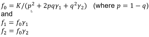

This is derived from the law of total probabilities which I will not show here.

Models for Dichotomous Traits

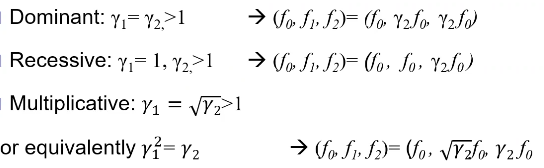
Note: multiplicative GRR ~= multiplicative OR
additive log(OR) -> multiplicative OR
Thus, multiplicative GRR model is most similar to the additive log(OR) model that we use in logistic regression