Three-Way Contingency Tables
In studying the association between two variables we should control for variables that may influence the relationship. To do so we can create K strata to control for a third variable.
When all involved variables are categorical, we can display the distribution of (E, D) as a contingency table at different levels of C.
The cross-section of tables are called partial tables. The 2-way table that displays the distribution of (E,D) disregarding C is called the E-D marginal table.
Partial tables can exhibit different association than the marginal tables (Simpson's Paradox); for this reason analyzing marginal tables can be misleading.
Simpson's Paradox occurs when an association between two variables is reversed upon observing a third variable.
Independence
In 1959, Mantel and Haenszel proposed a test for independence (between E and D) while adjusting for a third variable (C). This test statistic is called the Cochran-Mantel-Haenszel test statistic and is defined as:
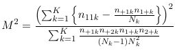
1. Under the conditional independence assumption (across all strata) M2 follows a chi-squared distribution with 1 degree of freedom.
2. M2 has good power against the alternative hypothesis of consistent patterns of association across strata.
If conditional independence assumption fails one might be interested in testing the assumption that OR is the same across the K tables. This could be done with the Breslow-Day Test for Homogeneity of Odds Ratios (reported by PROC FREQ in SAS).
title1 " Care and Infant survival in 2 clinics " ;
data care ;
input clinic survival $ count care ;
cards ;
1 died 3 0
1 died 4 1
1 lived 176 0
1 lived 293 1
2 died 17 0
2 died 2 1
2 lived 196 0
2 lived 23 1
run ;
proc freq data = care ;
table clinic * survival * care / cmh chisq relrisk ;
weight count ; run ;
Note that:
- The methods outlined here apply not only to situations where the classification variables are both responses (this will be explored in a later section)
- We will cover a way to test conditional independence based on Log-Linear models next
Log-Linear Models for S x R x K Tables
Every association between three variables can be coded with a different Log-Linear model. We will select among the association patters, using the deviance GoF statistic.
Saturated Model

The number of parameters: 1 + S + R + K + RK + SK + RSK
To reduce the number of parameters we impose linear constraints on the parameters. Consider the following examples:
Reference Coding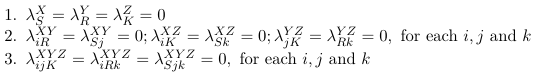
Effect Coding (Zero Sum Constraints)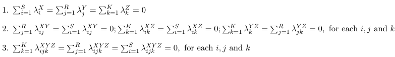
In the saturated model the number of parameters is:
1+(S - 1)+(R - 1)+(K −1)+(S −1)(R−1)+(S −1)(K −1)+(R−1)(K −1)+(S −1)(R−1)(K −1) = SRK
Note that with the saturated model we make no assumption regarding the association among variables.
Let's consider another model with all two-way interactions (no three-factor interaction):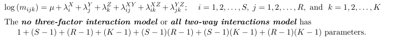
Under this model the association between X and Y is the same between different levels of Z; The association between X and Z is the same at different levels of Y; and the association between Z and Y is the same at different levels of X.
We can actually do the math and o serve that the Odds Ratio between X and Y (ORKXY) is the same at all levels of Z (it does not depend on k):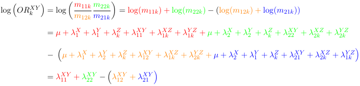
Mutual Independence Model

No interactions, the model assumes X, Y and Z are mutually independent.
The number of parameters will be: 1 + (S - 1) + (R - 1) + (K - 1)