Hypothesis Testing with GLM
Effect modification can be modeled with logistic regression by including interaction terms. A significant interaction term implies a departure from heterogeneity between groups.
Consider the following example were we wish to compare admission rates by sex per department: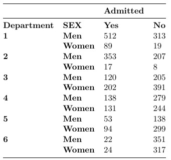
With summary of fit: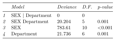
Which we observe only the saturated model fits the data well. To compare ORs across department we estimate the department specific odds from the saturated model:
ods select estimates ;
title1 ’ Estimated ODDS Ratio ( F vs M ) in each Department ’;
proc genmod data = one ;
class department SEX ;
model yes / total = SEX | department / link = logit dist = bin covb ;
estimate ’ SEX1 ’ SEX 1 -1 department * SEX 1 -1 0 0 0 0 0 0 0 0 0 0/exp;
estimate ’ SEX2 ’ SEX 1 -1 department * SEX 0 0 1 -1 0 0 0 0 0 0 0 0/exp;
estimate ’ SEX3 ’ SEX 1 -1 department * SEX 0 0 0 0 1 -1 0 0 0 0 0 0/exp;
estimate ’ SEX4 ’ SEX 1 -1 department * SEX 0 0 0 0 0 0 1 -1 0 0 0 0/exp;
estimate ’ SEX5 ’ SEX 1 -1 department * SEX 0 0 0 0 0 0 0 0 1 -1 0 0/exp;
estimate ’ SEX6 ’ SEX 1 -1 department * SEX 0 0 0 0 0 0 0 0 0 0 1 -1/exp;
run ;
The hypothesis tests we've encountered so far can be expressed in terms of linear combinations of the model parameters; However, other tests have to be carried out that may not be included in default output which requires a good understanding of the model.
For example, a few important properties we've seen so far:
- Differences between groups (Lecture 4)
Expressed as a linear combination:
1 × β1 + 0 × β2 + (−1) × β3 + 0 × β4 = 0 - Independence in 2 way tables defines by categorical variables X and Y
H0: X and Y are independent <-> H0: all λXYij = 0
HA: X and Y are dependent <-> HA: at least one λXYij != 0
Expressed as a linear combination:
λ11 = λ12 = λ21 = λ22 = 0
1 × λ11 + 0 × λ12 + 0 × λ21 + 0 × λ22 = 0
0 × λ11 + 1 × λ12 + 0 × λ21 + 0 × λ22 = 0
0 × λ11 + 0 × λ12 + 1 × λ21 + 0 × λ22 = 0
0 × λ11 + 0 × λ12 + 0 × λ21 + 1 × λ22 = 0 - Significance of parameters (Lecture 4)
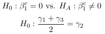
Expressed as a linear combination:
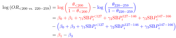
(For ordinal SBP): 0 × β0c + 1 × β1c + 0 × β2c = 0
(For SBP): γ1 + (−2) × γ2 + γ3 + 0 × γ4 = 0

In all cases the null hypothesis can be expressed as a linear combination of the parameters.