GLM for Count Data
Generalized linear models for count data are regression techniques available for modeling outcomes describing a type of discrete data where the occurrence might be relatively rare. A common distribution for such a random variable is Poisson.
The probability that a variable Y with a Poisson distribution is equal to a count value
$${ P(Y = y) = {{\lambda^y e^{-\lambda}} \over {y!}}} y = 0, 1, 2, ..., \infty $$
where λ is the average count called the rate
The Poisson distribution has a mean which is equal to the variance:
E(Y) = Var(Y) = \(\lambda\)
The mean number of events is the rate of incidence multiplied by time passed
Because of this assumption, the Poisson distribution also has the following properties:
- If Y_1 ~ Poisson(λ_1) and Y_2 ~ Poisson(λ_2) where Y_1 and Y_2 are the number of subjects in groups 1 and 2, then Y_1 + Y_2 ~ Poisson(λ_1 + λ_2)
- This generalizes to the situation of n groups as: Assuming n independent counts of Y_i are measured, if each Y_i has the same expected number of events λ then Y_1 + Y_2 + ... + Y_n ~ Poisson(nλ). In this situation λ is interpretable as the average number of events per group.
Poisson Regression as a GLM
To specify a generalized linear model we need (1) the distribution of outcome, (2) the link function, and (3) the variance function. For Poisson regression these are (1) Poisson, (2) Log, and (3) identity.
Let's consider a binomial example from a previous class where:
$$ Y_{ij} \approx Binomial(N_{ij}, λ_{ij}) $$
Given a variable Y ~ Binomial(n, p), where n is number of experiments and p the probability of success, this binomial distribution can be approximated well by the Poisson distribution with mean n*p.
So from that we can assume the distribution of Y also follows:
$$ Y_{ij} \approx Poisson(N_{ij} λ_{ij}) $$
and thus
$$ log(E(Y_{ij})) = log(N_{ij}) + log(\lambda_{ij}) $$
Since log(N_ij) is calculated from the data, we will proceed by modeling log(λ_ij) as a linear combination of the predictors:
$$ log{λ_{ij} } = μ + β_1X_{ij}^1 + β_2 X_{ij}^2 + . . . + β_k X_{ij}^k $$
The natural log is attractive as a link function for several reasons:
- The log link maps relative rates into additive effects
- With this link, parameters are readily interpretable as rate ratios, these ratios are called relative risks (risk ratios)
- The log link transforms positive values into the whole real link.
This the Poisson regression models extend the loglinear models; loglinear models are instances of Poisson regression.
Modeling Details
With the assumption
$$ E(Y_i) = N_i*λ_i $$
then using a log link we have:
$$ log(E(Y_{i})) = log(N_{i}) + log(\lambda_{i}) $$
Assuming we have a set of k predictors X1, X2, ..., Xk (continuous and/or ordinal and/or nominal), in Poisson regression one the linear predictors can be represented as:
$$ log{λ_i} = μ + β_1X_{i}^1 + β_2 X_{i}^2 + . . . + β_k X_{i}^k $$
We can represent the expected value as: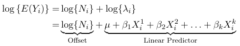
Where the term log(N_i) is called the offset. The offfset allows us to consider groups of different sizes in the model, but carries little value in terms of outcome.
In SAS we can use GENMOD to specify the Poisson distribution and an optional offset, but we must calculate the value ourselves.
proc genmod data = claims ;
class district car age ;
model C = district car age / offset = logN dist = poisson link = log obstats ;
estimate ’ district 1 vs . 4 ’ district 1 0 0 -1/ exp ;
run ;
In the results, the distribution of the chi-squared residuals (or deviance residuals) can be approximated by standard normal distribution. When the number of cells is large this assumption can be checked via a normal quantile plot, such as PROC UNIVARIATE; A linear pattern is evidence of a good fit.
Interpretation of Parameters
Interpretation is much the same as in a binomial model, we compare the rate of incidence in the reference group to that of the other groups:
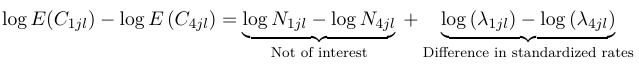
The most common use of a Poisson regression is in the analysis of time-to-event or survival. In cohort studies, the analysis of data usually involves estimation of disease during a defined period of observation; In this case the denominator of such a rate is measured in years of observation per person (person-years).
Over-dispersion in Poisson Regression
Over-dispersion occurs when the variance of the response exceeds the mean (nominal variance in Poisson); That is:
$$ var(Y) > E(Y) = n \pi (1 - \pi) $$
This can be the result of several phenomena:
- When the response is a random sum of independent variables, that is Y = R_1 + R_2 + ... + R_k where k is distributed as Poisson independent of R_i's
- When Y ~ Poisson(L), where L is random (this appears when there is inter-subject variability). The classical assumption is that L ~ Gamma(α, μ)
- When missing important covariates
- When the total population (N) is random rather than fixed